Spanish Fly for two - how they affect libido in women and men
Contents Biologically active additive based on an extract obtained from a beetle with a fly (or fly...
Types of costs; firm - its revenue and profit; profit maximization principle
Before proceeding with the analysis of production costs, we need to clarify what we mean by costs and how we will measure them. What items should be included in a firm's costs? Obviously, the costs include the wages of employees and employees of the firm and the rent for the office premises. What if the firm already owns office space and doesn't need to pay rent? And how should we view the funds that the firm spent two or three years ago (and cannot yet recoup) on equipment and R&D?
There are two approaches to cost analysis: accounting and economic. An economist looks at production costs differently from an accountant who is interested in a firm's balance sheet. Accountants tend to analyze the actual costs already incurred, as they have to keep track of assets and liabilities and assess the performance of the firm in the past. Actual costs include actual costs and depreciation charges for capital equipment, the amount of which is determined in accordance with tax legislation.
Economists and executives, on the contrary, are interested in the prospects of the firm. Οʜᴎ are concerned about upcoming costs and how to reduce them and increase profitability. Οʜᴎ, therefore, should be interested opportunity costs (see introductory topic) - the costs associated with lost opportunities to make the best use of the firm's resources. Opportunity costs include, but are not limited to, the explicit costs incurred by the firm.
Thus, when analyzing costs, an economist always proceeds from the fact that:
1) the reserves of resources available for involvement in production are limited;
2) there are several possibilities for the application of all resources and economic decisions always carry uncertainty;
3) all costs that affect supply have three characteristics: a) costs are associated with actions, not with things; b) they represent missed opportunities for specific decision makers; c) they are expected, based on marginal values, since opportunity costs involve additional costs.
Although opportunity costs are often hidden, they should always be taken into account when making economic decisions. The opposite is true with sunk costs - they are usually visible, but they are always ignored when making economic decisions.
sunk costs represent past and unreimbursed expenses. Because of their non-refundability, they do not influence the firm's decisions. For example, consider the purchase of special equipment, custom-designed by a factory. We assume that the equipment may only be used for the purpose for which it was originally intended and may not be remanufactured for an alternative use or sold to another firm. The cost of such equipment is irreversible, the opportunity cost of using it is zero. Perhaps it was not worth buying this equipment. It was of no use. However, today it does not matter, and these costs do not affect the decisions of the firm.
All costs are conditionally divided into external and internal. The cost of resources available to the firm itself is called internal. If the firm acquires resources from other firms, then this external costs. Internal the costs are equal to the monetary payments that could be received by the best use of this resource. Part of the profit is related to costs. There is a concept of economic and accounting profit. Accounting profit- the difference between total revenue (TR \u003d P * Q) and external costs. Economic profit is the difference between total revenue and opportunity costs for all resources. Normal profit is the profit that allows the company to stay in the industry. If opportunity costs exceed income (revenue), then the negative value of profit will be called the company's losses. General designation of costs WITH(from English cost - costs, expenses) →
C = F(Q). However, not all costs are the same. There are several types of costs in terms of their impact on output. In the short term, in the most general form, there are TS (total cost) - total costs, including fixed (FC) and variable costs ( VC). Fixed costs do not depend on the volume of output and may also occur when no output is produced at all, for example, rent, payment of interest on a loan, etc. Variable costs change with changes in output. These are the costs for the purchase of raw materials, materials, electricity, etc.
Thus: TC = FC + VC. Average cost - AC = TS / Q.
And FC- average fixed costs. AFC = FC / Q. AVC are average variable costs. AVC = VC/Q. Hence, AC (ATS) \u003d AFC + AVC.
Marginal or marginal cost (MC). Marginal cost is the increase in costs resulting from the production of one additional unit of output.. MS= ∆TC/ ∆Q. Or MC=(TC)" = (dFC/dQ) + (dVC/dQ) = 0 + (dVC/dQ). Because fixed costs do not change with changes in the firm's output. Marginal cost is determined by the growth of only variables . Graphically, the relationship of costs will look like this:

As we have determined. But , where W is wages and , where L is the value of the variable factor. Then ![]()
What explains this behavior of the curves? It is assumed that if there is at least one fixed resource, the quantity of which cannot be changed, then with an increase in variable costs for other resources, the average productivity of variable resources first increases (average variable costs fall), and then, starting from a certain volume of output, productivity decreases ( average variable costs rise).
The form of the curve of average total costs is determined, firstly, by the form of the curve of average variable costs AVC, built on the basis of the law of diminishing productivity; secondly, the shape of the average fixed cost curve, despite the fact that AFC = ATC-AVC.
If average cost increases, then marginal cost is greater than average cost. If average cost is decreasing, then marginal cost is lower than average cost. At the lowest point of the average cost curve, marginal cost will equal average cost.
Using the isoquant method to determine the producer's equilibrium.
The problem of finding the optimal output for a given producer with variable inputs can be approached graphically using the isoquant method. Let us assume that two factors of production are used in production: labor and capital (hours of use of labor and machinery or equipment). The price of labor is equal to the wage rate (w). The price of capital is equal to the rent for equipment (r). Lines reflecting all possible combinations of labor and capital, having a single total cost, are called isocosts. The isocost equation: TC= wL + r K. Isocost is a straight line, each point, which shows what combination of two factors of production a firm can acquire at its own expense. The equilibrium of the producer will be established at the point where the isocost touches the isoquant. The slope of the isoquant and isocost is the same here.
In the long run, for a given output, the firm achieves an equilibrium in the application of inputs, maximizing profits and minimizing costs, when any replacement of one input by another does not lead to a decrease in unit costs. It happens when MP K / r = MP L / w. That is, since in the long run all input factors of production can be changed, then at a given volume of production, the firm reaches an equilibrium in the use of input factors of production and minimizes costs when any replacement of one factor by another does not lead to a decrease in unit costs. This is what happens when the above equality is satisfied.
But everything that has been said above refers precisely to the volume of output already given. And when will the firm begin to reduce or increase the output of finished products? That is, in the broadest sense, an enterprise can also change the size of production itself in the long run. Take for example a small manufacturing enterprise, ĸᴏᴛᴏᴩᴏᴇ, with minimal production capacity, begins to expand its output. Initially, the expansion of output is accompanied by a decrease in average total costs. Then the introduction of new capacities leads to an increase in average total costs. Then The long run average cost curve (LAC) of an individual firm is made up of segments of the short run average total cost (SATC) in relation to the size of those enterprises that are built. The LAC curve shows the lowest cost of producing a unit of output at which any output can be achieved, provided that the firm has had sufficient time at its disposal to make all the necessary changes in the size of enterprises. The LAC curve is called the firm's plan curve (the choice curve).
|

The arcuateness of the LAC curve is explained by the positive and negative effects of scale. Positive economies of scale - the effect of mass production or economies of scale (descending part of the curve). With the growth of the size of the enterprise, a number of factors reduce the ATS: 1) specialization of labor; 2) specialization of managerial personnel; 3) efficient use of capital; 4) production of by-products and waste disposal. The negative effect of scale is associated with certain managerial difficulties in controlling and coordinating the actions of a large number of subdivisions of an expanded enterprise. There are different types of long run cost curves.
This section will not consider the behavior of a perfectly competitive firm as a market structure. We are only talking about a classic firm that forms its offer on the market as a seller. The firm's supply curve shows how much output the firm will produce at each possible price. As we saw above, firms will increase output up to the point where price equals marginal cost, but curtail production if the price is below average variable cost. Therefore, for non-zero output, the supply curve of any firm coincides with that part of the MC line that lies above the AVC curve, that is, above the point of minimum average variable costs. Anything above the bankruptcy point corresponds to the prices that the firm could offer. An increase in the market price generally encourages firms already in the market to increase output.
Factors influencing the offer:
1) the prices of resources used in the production of this firm;
2) the level of technology (the use of more advanced technology will lead to a reduction in costs and an increase in production volume, that is, the ATC, AVC, MC curves will shift upwards);
3) change in prices for other goods related to the data and change in the number of producers of these goods;
4) the policy of the state in relation to the producers of this product.
There is an individual offer and an offer on the market as a whole. Let all supply factors except price remain unchanged. There are not one, but two sellers on the market for this product. Differences in their offer are due to the conditions of their individual production. The market volume of supply will be formed by horizontal summation of the individual supply volumes of each seller at a given price.
In practice, the expansion of the volume of production entails a change in the prices of the resources used. Another situation is also possible: the expansion of the production of goods stimulates the growth of the production of resources, which in turn can reduce costs. All these situations and others will be considered in the analysis of the resource market.
Firms industries produce products in volumes corresponding to the points of minimum values of their curves of average total costs in the short run (SATC). For all firms in an industry, their marginal cost of production equals the price of the good.
The firms in the industry also produce output in volumes corresponding to the minimum points of their average cost curves in the long run. When all firms in an industry operate at minimum cost in the long run, that is, all three equilibrium conditions are satisfied, then the industry is said to be in equilibrium. This means that at a given level of technology development and constant prices for economic resources, each firm in the industry completely exhausts its internal reserves for optimizing production and minimizes its costs. If neither the level of technology nor the prices of factors of production change, then any attempt by the firm to increase (decrease) production volumes will lead to losses.
The manual is presented on the website in an abbreviated version. In this version, tests are not given, only selected tasks and high-quality tasks are given, theoretical materials are cut by 30% -50%. I use the full version of the manual in the classroom with my students. The content contained in this manual is copyrighted. Attempts to copy and use it without indicating links to the author will be prosecuted in accordance with the legislation of the Russian Federation and the policy of search engines (see the provisions on the copyright policy of Yandex and Google).
We have already defined that the market is a set of rules, using which buyers and sellers can interact with each other and carry out transactions (transactions). Over the history of the development of economic relations between people, markets are constantly undergoing transformations. For example, 20 years ago there was not the abundance of electronic markets that are available to the consumer now. Consumers could not buy a book, household appliances, or shoes by simply opening an online store website and making a few clicks.
At the time when Adam Smith began to talk about the nature of markets, they were arranged something like this: most of the goods consumed in European economies were produced by a multitude of manufactories and artisans who used mainly manual labor. The firm was very limited in size, and employed only a few dozen workers at the most, and most often 3-4 workers. At the same time, there were quite a lot of such manufactories and artisans, and they were producers of fairly homogeneous goods. That variety of brands and types of goods that we are used to in the modern consumer society did not exist then.
These signs led Smith to conclude that neither consumers nor producers have bargaining power, and the price is set freely by the interaction of thousands of buyers and sellers. Observing the features of the markets in the late 18th century, Smith came to the conclusion that buyers and sellers are guided towards equilibrium by an "invisible hand". The characteristics that were inherent in the markets at that time, Smith summarized in the term "perfect competition" .
A perfectly competitive market is a market with many small buyers and sellers selling a homogeneous product under conditions where buyers and sellers have the same information about the product and each other. We have already discussed the main conclusion of Smith's "invisible hand" hypothesis - a perfectly competitive market is able to provide an efficient allocation of resources (when a product is sold at prices that exactly reflect the firm's marginal cost of producing it).
Once upon a time, most markets really looked like perfect competition, but in the late 19th and early 20th centuries, when the world became industrialized, and monopolies formed in a number of industries (coal mining, steel production, railway construction, banking), it became clear that the model of perfect competition is no longer suitable for describing the real state of affairs.
Modern market structures are far from the characteristics of perfect competition, so perfect competition is currently an ideal economic model (like an ideal gas in physics), which is unattainable in reality due to the numerous forces of friction.
The ideal model of perfect competition has the following characteristics:
Under these conditions, the market is able to allocate resources and goods efficiently. The criterion for the efficiency of a competitive market is the equality of prices and marginal costs.
Why does allocative efficiency arise when prices equal marginal cost and is lost when prices do not equal marginal cost? What is market efficiency and how is it achieved?
To answer this question, it suffices to consider a simple model. Consider potato production in an economy of 100 farmers whose marginal cost of potato production is an increasing function. The 1st kilo of potatoes costs $1, the 2nd kilo of potatoes costs $2, and so on. None of the farmers has such differences in the production function that would allow him to gain a competitive advantage over the rest. In other words, none of the farmers have bargaining power. All potatoes sold by farmers can be sold at the same price, determined in the market for balances of general demand and total supply. Consider two farmers: farmer Ivan produces 10 kilograms of potatoes per day at a marginal cost of $10, and farmer Michael produces 20 kilograms at a marginal cost of $20.
If the market price is $15 per kilogram, then Ivan has an incentive to increase potato production because each additional product and kilogram sold earns him an increase in profits, as long as his marginal cost does not exceed $15. For similar reasons, Mikhail has an incentive to reduction in production volumes.
Now let's imagine the following situation: Ivan, Mikhail, and other farmers initially produce 10 kilograms of potatoes, which they can sell for 15 rubles per kilogram. In this case, each of them has incentives to produce more potatoes, and the current situation will be attractive for the arrival of new farmers. Although each of the farmers has no influence on the market price, their joint efforts will lead to a fall in the market price to a level until the opportunities for additional profit for each and every one are exhausted.
Thus, thanks to the competition of many players in conditions of complete information and a homogeneous product, the consumer receives the product at the lowest possible price - at a price that only breaks the marginal cost of the producer, but does not exceed them.
Now let's see how equilibrium is established in the perfectly competitive market in graphical models.
The equilibrium market price is established in the market as a result of the interaction of supply and demand. The firm accepts this market price as given. The firm knows that at this price it will be able to sell as many goods as it likes, so there is no point in lowering the price. If the firm raises the price of a product, it will not be able to sell anything at all. Under these conditions, the demand for the product of one firm becomes perfectly elastic:
The firm takes the market price as given, i.e. P = const.
Under these conditions, the firm's revenue schedule looks like a ray coming out of the origin:

This is easy to prove:
MR = TR Q ′ = (P * Q) Q ′
Because the P = const, P can be taken out of the sign of the derivative. As a result, it turns out
MR = (P * Q) Q ′ = P * Q Q ′ = P * 1 = P
MR is the tangent of the slope of the straight line TR.
A perfectly competitive firm, like any firm in any market structure, maximizes total profit.
A necessary (but not sufficient condition) for maximizing the firm's profit is the zero derivative of profit.
R Q ′ = (TR-TC) Q ′ = TR Q ′ - TC Q ′ = MR - MC = 0
Or MR=MC
That is MR=MC is another entry for the profit condition Q ′ = 0.
This condition is necessary but not sufficient for finding the maximum profit point.
At the point where the derivative is equal to zero, there may be a minimum of profit along with a maximum.
A sufficient condition for maximizing the firm's profit is to observe the neighborhood of the point where the derivative is equal to zero: to the left of this point, the derivative must be greater than zero, to the right of this point, the derivative must be less than zero. In this case, the derivative changes sign from plus to minus, and we get a maximum, not a minimum, of profit. If in this way we have found several local maxima, then to find the global profit maximum, you should simply compare them with each other and choose the maximum profit value.
For perfect competition, the simplest case of profit maximization looks like this:

More complex cases of profit maximization will be discussed graphically in the appendix in the chapter.
We realized that a necessary (but not sufficient) condition for maximizing the firm's profit is the equality P=MC.
This means that when MC is an increasing function, the firm will choose points on the MC curve to maximize profits.
But there are situations when it is beneficial for the firm to leave the industry, instead of producing at the point of maximum profit. This happens when the firm, being at the point of maximum profit, cannot cover its variable costs. In this, the firm incurs losses that exceed fixed costs.
The firm's optimal strategy is to exit the market, because in this case it receives losses exactly equal to fixed costs.
Thus, the firm will stay at the point of maximum profit, and not leave the market when its revenue exceeds variable costs, or, equivalently, when its price exceeds average variable costs. P>AVC
Let's look at the chart below:

Of the five marked points where P=MC, the firm will remain in the market only at points 2,3,4. At points 0 and 1, the firm will choose to leave the industry.
If we consider all possible positions of the line P, we will see that the firm will choose points lying on the marginal cost curve that will be higher than AVC min.
Thus, the competitive firm's supply curve can be plotted as the portion of MC above AVC min.
This rule is applicable only for the case when the curves MC and AVC are parabolas. Consider the case where MC and AVC are straight lines. In this case, the total cost function is a quadratic function: TC = aQ 2 + bQ + FC
Then ![]()
MC = TC Q ′ = (aQ 2 + bQ + FC) Q ′ = 2aQ + b
We get the following graph for MC and AVC:

As can be seen from the graph, when Q > 0, the MC graph always lies above the AVC graph (because the straight line MC has an angle of inclination 2a, and the straight line AVC slope angle a.
Recall that in the short run, the firm necessarily has both variable and fixed factors. So, the costs of the firm consist of a variable and a fixed part:
TC = VC(Q) + FC
The firm's profit is p \u003d TR - TC \u003d P * Q - AC * Q \u003d Q (P - AC)

At the point Q* The firm achieves maximum profit because it P=MC(necessary condition), and profit changes from increasing to decreasing (sufficient condition). On the graph, the profit of the firm is depicted as a shaded rectangle. The base of the rectangle is Q*, the height of the rectangle is (P-AC). The area of the rectangle is Q * (P - AC) = p
That is, in this variant of equilibrium, the firm receives economic profit and continues to operate in the market. In this case P > AC at the point of optimal release Q*.
Consider the equilibrium where the firm earns zero economic profit

In this case, the price at the optimum point is equal to the average cost.
A firm can earn even negative economic profits and still continue to operate in the industry. This happens when, at the point of optimum, the price is lower than the average, but higher than the average variable costs. The firm, even receiving economic profit, covers the variable and part of the fixed costs. If the firm leaves, then it will bear all the fixed costs, so it continues to operate in the market.

Finally, the firm exits the industry when, at optimal output, its revenue does not even cover variable costs, that is, when P< AVC

Thus, we have seen that a competitive firm can earn positive, zero, or negative profits in the short run. The firm leaves the industry only when, at the point of optimal output, its revenue does not even cover variable costs.
The difference between the long run and the short run is that all factors of production for the firm are variable, that is, there are no fixed costs. Just as in the short run, firms can freely enter and exit the market.
Let us prove that in the long run the only stable state of the market is one in which the economic profit of each firm tends to zero.
Let's consider 2 cases.
Case 1 . The market price is such that firms earn a positive economic profit.

What will happen to the industry in the long run?
Since information is open and publicly available, and there are no market barriers, the presence of positive economic profits for firms will attract new firms to the industry. Entering the market, new firms shift the market supply to the right, and the equilibrium market price falls to a level at which the opportunity for positive profits has not been completely exhausted.
Case 2 . The market price is such that firms earn negative economic profits.

In this case, everything will happen in the opposite direction: since firms earn negative economic profit, some firms will leave the industry, supply will decrease, the price will rise to a level at which the economic profit of firms will not become zero.
A perfectly competitive firm is a firm operating in a perfectly competitive market. A perfectly competitive market is a market structure characterized by price competition between firms unable to exert any influence on the market price. Among the specific features inherent in it, it should be noted that a perfectly competitive firm:
1) cannot influence the market price;
2) takes the market price as given.
Therefore, with perfect competition, the interaction between firms is devoid of strategic behavior, i.e. the company does not take into account the reaction of its competitors to the decisions it makes, and the essence of its behavior is reduced to adapting the emerging market situation.
The offer of a perfectly competitive firm in the short run. Since a perfectly competitive firm is not able to influence the market price, then for it the implementation of the principle of profit maximization is associated with the choice of the volume of supply. It should be such that the marginal cost of production is equal to the market price of a unit of output. Given that within the framework of the technology used by the firm, the level of marginal costs is determined by the characteristics of the production function, it becomes obvious that the volume of supply of the firm will depend on the level of the market price.
A) the case of profit maximization
A firm always maximizes total profit at an output for which marginal revenue equals marginal cost. As long as marginal revenue exceeds marginal cost, the total profit function will rise and the firm will increase its supply.
B) a case of self-sufficiency
If the market price drops to the level of the minimum average cost, the firm will continue to produce, operating on a self-sufficiency basis. In this case, not receiving economic profit, the firm will actually have some accounting profit. Therefore, the firm always carries out production for which the total cost is minimally greater than the total revenue.
C) loss minimization case
The firm always minimizes short-run losses by stopping production if the price falls below average variable cost. In the event of a cessation of production, the losses of the firm will amount to an amount equal to the total fixed costs.
A perfectly competitive firm's supply curve in the short run is the portion of its marginal cost curve above the minimum average variable cost.
The offer of a perfectly competitive firm in the long run. In the long run, a firm can change all factors and even leave the industry, while other firms can enter it, which determines the nature of establishing long-term market equilibrium.
In the long run, perfectly competitive firms produce at the lowest long-run average cost and earn no economic profit.
A perfectly competitive firm's long-run supply curve represents the portion of the upward segment of its long-run marginal cost curve that lies above the intersection with the long-run average cost curve..
Analyzing the mechanism that regulates the number of firms in the industry, one should take into account the realities of economic practice. Thus, given the difficulties of capital flow, this mechanism works better for expansion rather than contraction. In addition, even knowing that economic profit will be zero in the long run, firms can enter the industry for a variety of reasons:
The desire to get high profits in the short term;
Differences in real costs;
Difficulties in establishing long-term equilibrium;
availability of accounting profit.
The offer of a perfectly competitive industry.Industry supply in the short run . Industry (market) offer represents the volume of output carried out by all firms in the industry. If equilibrium is reached in the industry, then the supply of each firm in the industry in the short run will be represented by its marginal cost curve.
The short-run market supply curve of a perfectly competitive industry is the sum of the short-run supply curves of the individual firms.
The principle of summing the supply curves of firms to determine the industry supply curve is applicable only to the extent that the prices of the variable factors used in the industry remain unchanged. Since an increase in industry supply will lead to an increase in demand for variable factors and may cause an increase in prices for them, in reality, building an industry supply curve is not reduced to adding the supply curves of individual firms. The short-term industry supply curve itself will be determined by such factors as:
1) the number of firms in the industry;
2) the average size of firms in the industry;
3) prices of variable resources used by the industry;
4) technologies used in the industry.
Industry supply in the long run. The expansion or contraction of the industry does not affect market equilibrium prices, since it inevitably returns to the level of the minimum long-run average cost. This means that the long-run industry supply curve is perfectly elastic and should be represented by a horizontal straight line. However, this assumption is valid only in the case of constant prices for factors of production. But since the prices of factors can change under the influence of demand for them, the position of the industry's long-run supply curve will depend on the extent to which a change in the industry's output has affected the prices of the factors of production used by the industry. Depending on the nature of this influence, industries are distinguished:
1) with fixed costs;
2) with growing costs;
3) with decreasing costs
Free competition means that, firstly, there are many independent firms on the market that independently decide what and how much to produce. Secondly, access to the market is not limited to anyone and nothing, and exit from it is also free. This implies the opportunity for every citizen to become a free entrepreneur and apply his labor and material resources in the sector of the economy that interests him. Buyers must be free from any discrimination and be able to buy goods and services in any market. Thirdly, products of a certain purpose are the same in terms of their most important properties. Fourth, firms have no part in controlling market prices.
Perfect Competition is a market structure in which many firms sell a standardized product and no single firm has a large enough market share to influence its price.
Continuous confrontation acts as a force that directs the activities of all agents of the market. Competition as a market regulator naturally affects three phenomena: a) changes in prices of buyers and sellers; b) an unstable ratio of supply and demand associated with areas of excess and lack of goods; c) the deviation of the market price from the equilibrium point.
The law of competition has a stronger effect on the behavior of market participants than the laws of supply and demand. Free competition, as it were, forces excessively high and very low prices to move towards the equilibrium point. This centripetal movement leads, ultimately, to the equality of the opposing sides. The direct involvement of market competitiveness in the formation of an equilibrium price and an equilibrium quantity of goods dictates competitive game rules(behavior).
7.3. Monopoly: place and role in the market
Monopoly - this is the exclusive right of the state, enterprise, organization, trader to carry out any economic activity. This means that, by its nature, a monopoly is the direct opposite of free competition.
The “pure monopoly” market model is characterized by the presence of only one firm producing a product for which there are no close substitutes, i.e. a unique product, the firm exercises significant control over the price of its product. By adjusting the price by changing the supply of the product, the firm does everything to prevent a new firm from entering the industry of its activity, i.e., blocks its industry. Commercial advertising of the product is almost non-existent.
A situation in which there are many sellers in the market and only one buyer of a product is called monopsony (i.e. monopoly of one buyer)
In different countries in different periods in the economy there are different types of monopolies. This type of market structure can be classified according to the degree of coverage of the economy, the nature and causes of occurrence.
The rules of behavior of monopolistic associations in the market differ from those inherent in free competition by a fundamentally different approach to pricing. Monopolists conquer the market in order to collect a kind of tribute from economic entities dependent on them with the help of the prices they set. Thus, they receive much higher incomes compared to the average level established in the national economy.
Unlike participants in a competitive market, monopoly firms themselves and at their own discretion set the market price for their products.
There are four rules for setting a monopoly price.
First rule. Firm installs monopoly high price on their products in excess of the social value or the possible equilibrium price. This is achieved by the fact that monopolists deliberately create a deficit zone, reducing production and artificially creating increased consumer demand.
Second rule. Monopsony sets exclusive low prices for purchased goods. Lowering the price compared to the social value or the possible equilibrium price is achieved by artificially creating a zone of excess production. In this case, the monopsony deliberately reduces the purchase of goods, due to which their supply exceeds the monopolistic demand.
The demand for the products of an individual competitive firm whose sales volume has no effect on the change in market price reflects a demand line that has a horizontal shape, or a perfectly elastic demand line. It shows that a firm will sell any number of goods and services at the same price (P), which is determined by the general industry supply and demand.
Third rule A firm that is both a monopoly and a monopsony doubles the tribute it collects through so-called price scissors. We are talking about monopoly high and monopoly low prices, the levels of which move away from each other like diverging scissor blades. This behavior is typical for many manufacturing enterprises, which, in the context of inflation, raise prices for finished products several times more than prices in the extractive industries.

Contents Biologically active additive based on an extract obtained from a beetle with a fly (or fly...

Ekaterina MirimanovaSystem minus 60. Revolution System minus 60 with Ekaterina Mirimanova"System minus 60. Revolution"...

Heaviness and bloating are the causes of both ordinary overeating and more serious problems with the digestive tract....

The second blood type, Rh-negative, appeared many years ago, when a person stopped being a hunter, and ...

PSYCHOLOGICAL ASPECTS OF THE PHENOMENON OF ANOREXIA (EXPERIMENTAL STUDY) T. V. Tarasova, E. V. Arsent'eva V...

Contents Due to the fact that the skin in this area is thin, it is more prone to the appearance of various kinds of spots. Redness under...
vseslav Sat, 10/17/2015 - 20:50 Vasileostrovskaya station is one of the oldest stations...

Most often, the goat mushroom (Suillus bovinus) is referred to in the everyday speech of mushroom pickers as a goat. This tubular...

Every person has had dreams at least once in their life. Many do not attach any importance to them, but some ...
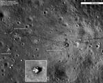
Daedalus (crater). Diameter: 93 km Depth: 3 km (NASA photo) The moon has attracted people's attention since ancient times. In II...

The United States celebrates President's Day on the third Monday in February. Until the 70s, the celebrations were timed to...

On the day of the last call, I want to say just one word to my beloved head teacher: “Thank you.” But how much is...
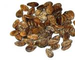
Watermelon is considered a tasty and healthy berry, its seeds are especially useful. Small, dark brown or...

“The development of speech in children of 6 years old” A child is not born with an established speech. It is not possible to give a definitive answer to...

Although obesity in itself is not a specific disease, it becomes a breeding ground for ...

Parsley is a green plant with a spicy and rich aroma. The most common...