What is possible and not possible during the Nativity Fast?
In 2018, the Nativity Fast will begin on November 28. During this period, Orthodox believers prepare to celebrate Christmas...
The main feature of costs in the long run is the fact that they are all variable in nature - the firm can increase or reduce capacity, and it also has enough time to decide to leave a given market or enter it by moving from another industry. Therefore, in the long run, average fixed and average variable costs are not distinguished, but average costs per unit of production (LATC) are analyzed, which in essence are also average variable costs.
To illustrate the situation with costs in the long run, consider a conditional example. Some enterprise expanded over a fairly long period of time, increasing its production volumes. The process of expanding the scale of activity will be conditionally divided into three short-term stages within the analyzed long-term period, each of which corresponds to different enterprise sizes and volumes of output. For each of the three short-term periods, short-term average cost curves can be constructed for different enterprise sizes - ATC 1, ATC 2 and ATC 3. The general average cost curve for any volume of production will be a line consisting of the outer parts of all three parabolas - graphs of short-term average costs.
In the example considered, we used a situation with a 3-stage expansion of the enterprise. A similar situation can be assumed not for 3, but for 10, 50, 100, etc. short-term periods within a given long-term period. Moreover, for each of them you can draw the corresponding ATS graphs. That is, we will actually get a lot of parabolas, a large set of which will lead to the alignment of the outer line of the average cost graph, and it will turn into a smooth curve - LATC. Thus, long-run average cost (LATC) curve represents a curve that envelops an infinite number of short-term average production cost curves that touch it at their minimum points. The long-run average cost curve shows the lowest cost per unit of production at which any level of output can be achieved, provided that the firm has time to change all factors of production.

In the long run there are also marginal costs. Long Run Marginal Cost (LMC) show the change in the total amount of costs of the enterprise in connection with a change in the volume of output of finished products by one unit in the case when the company is free to change all types of costs.
The long-run average and marginal cost curves relate to each other in the same way as the short-run cost curves: if LMC lies below LATC, then LATC falls, and if LMC lies above laTC, then laTC rises. The rising portion of the LMC curve intersects the LATC curve at the minimum point.

There are three segments on the LATC curve. In the first of them, long-term average costs are reduced, in the third, on the contrary, they increase. It is also possible that there will be an intermediate segment on the LATC chart with approximately the same level of costs per unit of output at different values of output volume - Q x. The arcuate nature of the long-term average cost curve (the presence of decreasing and increasing sections) can be explained using patterns called positive and negative effects of increased scale of production or simply scale effects.
The positive effect of scale of production (the effect of mass production, economies of scale, increasing returns to scale of production) is associated with a decrease in costs per unit of production as production volumes increase. Increasing returns to scale of production (positive economies of scale) occurs in a situation where output (Q x) grows faster than costs rise, and therefore the enterprise's LATC falls. The existence of a positive effect of scale of production explains the descending nature of the LATS graph in the first segment. This is explained by the expansion of the scale of activity, which entails:
1. Increased labor specialization. Labor specialization presupposes that diverse production responsibilities are divided among different workers. Instead of carrying out several different production operations at the same time, which would be the case with a small-scale enterprise, in conditions of mass production each worker can limit himself to one single function. This results in an increase in labor productivity and, consequently, a reduction in costs per unit of production.
2. Increased specialization of managerial work. As the size of an enterprise grows, the opportunity to take advantage of specialization in management increases, when each manager can focus on one task and perform it more efficiently. This ultimately increases the efficiency of the enterprise and entails a reduction in costs per unit of production.
3. Efficient use of capital (means of production). The most efficient equipment from a technological point of view is sold in the form of large, expensive kits and requires large production volumes. The use of this equipment by large manufacturers allows them to reduce costs per unit of production. Such equipment is not available to small firms due to low production volumes.
4. Savings from using secondary resources. A large enterprise has more opportunities to produce by-products than a small company. A large firm thus makes more efficient use of the resources involved in production. Hence the lower costs per unit of production.
The positive effect of scale of production in the long run is not unlimited. Over time, the expansion of an enterprise can lead to negative economic consequences, causing a negative effect of scale of production, when the expansion of the volume of a company's activities is associated with an increase in production costs per unit of output. Diseconomies of scale occurs when production costs rise faster than production volume and, therefore, LATC rises as output increases. Over time, an expanding company may encounter negative economic facts caused by the complication of the enterprise management structure - the management floors separating the administrative apparatus and the production process itself are multiplying, top management turns out to be significantly removed from the production process at the enterprise. Problems arise related to the exchange and transmission of information, poor coordination of decisions, and bureaucratic red tape. The efficiency of interaction between individual divisions of the company decreases, management flexibility is lost, control over the implementation of decisions made by the company's management becomes more complicated and difficult. As a result, the operating efficiency of the enterprise decreases and average production costs increase. Therefore, when planning its production activities, a company needs to determine the limits of expanding the scale of production.
In practice, cases are possible when the LATC curve is parallel to the x-axis at a certain interval - on the graph of long-term average costs there is an intermediate segment with approximately the same level of costs per unit of output for different values of Q x. Here we are dealing with constant returns to scale of production. Constant returns to scale occurs when costs and output grow at the same rate and, therefore, LATC remains constant at all output levels.
The appearance of the long-term cost curve allows us to draw some conclusions about the optimal enterprise size for different sectors of the economy. Minimum effective scale (size) of an enterprise- the level of output, starting from which the effect of savings due to an increase in the scale of production ceases. In other words, we are talking about such values of Q x at which the company achieves the lowest costs per unit of production. The level of long-term average costs determined by the effect of economies of scale affects the formation of the effective size of the enterprise, which, in turn, affects the structure of the industry. To understand, consider the following three cases.

1. The long-term average cost curve has a long intermediate segment, for which the LATC value corresponds to a certain constant (Figure a). This situation is characterized by a situation where enterprises with production volumes from Q A to Q B have the same cost. This is typical for industries that include enterprises of different sizes, and the level of average production costs for them will be the same. Examples of such industries: wood processing, timber industry, food production, clothing, furniture, textiles, petrochemical products.
2. The LATC curve has a fairly long first (descending) segment, in which there is a positive effect of production scale (Figure b). The minimum cost is achieved with large production volumes (Q c). If the technological features of the production of certain goods give rise to a long-term average cost curve of the described form, then large enterprises will be present in the market for these goods. This is typical, first of all, for capital-intensive industries - metallurgy, mechanical engineering, automotive industry, etc. Significant economies of scale are also observed in the production of standardized products - beer, confectionery, etc.
3. The falling segment of the long-term average costs graph is very insignificant; the negative effect of scale of production quickly begins to work (Figure c). In this situation, the optimal production volume (Q D) is achieved with a small volume of output. If there is a large-capacity market, we can assume the possibility of the existence of many small enterprises producing this type of product. This situation is typical for many sectors of the light and food industries. Here we are talking about non-capital-intensive industries - many types of retail trade, farms, etc.
Goals and objectives solved by a company when entering the market in a short-term time interval.
The firm evaluates its behavior as a business unit by comparing various types of income and costs. This is especially true for the behavior of a company in the short term. When entering the market, a company asks the following basic questions:
Should the product be manufactured and brought to market?
How much (what quantity) should the product be produced?
What profit or loss will the firm receive from selling this quantity of product?
The answer to the first question is yes, if as a result of the production and sale of a certain amount of products, positive economic profit, or losses, which in their magnitude will be less than fixed costs (TFC). At zero output, the firm incurs losses equal to TFC.
Answer to the second question: it is necessary to produce such a quantity of a product, the sale of which on the market provides the company with maximum profits or minimum losses.
Answer to the third question: it is necessary to consider specific situations of the relationship between income and costs in which maximizing profits or minimizing losses is possible.
9.6.Effect of scale and firm costs over a long-term time interval.
In the long run all the firm's resources are variable. A company can hire new equipment, rent new workshops, change the composition of management personnel, or use new production technology.
The lack of permanent resources in the long term leads to the fact that the difference between fixed and variable costs disappears. Analysis of the long-term activities of the company is carried out through consideration of the dynamics long-run average cost(LATC). And the main goal of the company in the area of costs can be considered the organization of production of the “required scale”, providing a given volume of production with minimum average costs.
Scope of the company's activities– dependence of the increase in production volume on the increase in the use of all factors of production over a long-term time interval.
Economies of scale– savings due to an increase in the scale of the firm’s activities, manifested in a reduction in long-term average costs.
To construct long-run average costs, assume that
a firm can organize production of three sizes: small, medium and large, each of which has its own short-term average cost curve (SATC1, SATC2, SATC3, respectively), as shown in Fig. 5.
Fig.5 Long-run average cost curve.
The choice of a particular project will depend on estimates of projected market demand on the company's products and on what capacity is needed to provide it.
If the forecasted demand corresponds to Q1, then the firm will prefer to create small production, since its average costs in this case will be significantly lower than at larger enterprises. As can be seen in Figure 5, ATC1(Q1) If demand is expected to be Q2, then project 2 (medium enterprise) will be most preferable, providing lower costs, or ATC2(Q2) Combining the portions of the three short-run cost curves that provide the optimal production size for each output shows us long-run average cost curve companies. In Figure 5 it is represented by a solid line. Long-Run Average Cost Curve
shows the minimum cost per unit of output produced at each possible output level. If the number of possible sizes (Q1, Q2,...Qn) approaches infinity (), then the long-term average cost curve becomes flatter, as shown in Figure 6. Fig. 6 Long-term average cost curve for an unlimited number of possible enterprise sizes In this case, all points on the LATC curve are lowest average cost for a given volume of production, provided that the firm has enough time to change all the necessary resources. In the short term, all costs are divided into fixed and variable. Fixed costs
(FC
)
– these are cash costs that do not depend on the volume of output (costs of operating equipment, buildings, structures, interest on loans, rental payments, insurance premiums, management salaries, security, etc.) Fixed costs are mandatory and remain, even if the company does not produce anything, therefore, on the graph, fixed costs are expressed as a straight line parallel to the x-axis (Fig. 5.1). Variable costs
(V.C.
)
- These are monetary costs that change with the volume of product output. They include the costs of raw materials, auxiliary materials, energy, worker labor, etc. Variable costs change in proportion to production output, therefore, on the graph, the variable cost curve is an ascending line (Fig. 5.1). The sum of fixed and variable costs forms the total, gross or total costs of production. General costs
(TS
)
- this is the totality of all the enterprise’s costs for the production and sale of products: The total cost curve completely repeats the variable cost line, but is shifted upward from it by the amount of fixed costs (Fig. 5.1). To make management decisions, producers must know not only the total amount of costs, but also their value per unit of production - average costs
.
There are three types of average costs: average fixed costs; average variable and average total costs. Average fixed costs (AFC)
is the ratio of fixed costs to output: Average variables
costs (AVC)
is the ratio of variable costs to the volume of output: Average Total Cost (AC)
can be calculated using the formulas: The additional costs associated with increasing production per unit are called marginal (MC)
:
Since FC = const, there is no relationship between fixed and marginal costs. Therefore, marginal costs are expressed by the formula: At any given time, different firms have a certain size. Within these dimensions, costs change in accordance with the model described for the short term. In the long run, a firm can change all its resources, so all factors of production become variable. Since in LR the firm can change all its parameters, it seeks to increase output by reducing long-run average cost (LAC).
Long Run Marginal Cost (LMC)
- this is an increase in production costs in conditions when the manufacturer has the opportunity to change the size of the enterprise. If LMC< LAC, то долгосрочные средние
издержки уменьшаются. Если же LMC >LAC, then average costs increase. When LAC = LMC, then long-run average cost reaches its minimum. Production costs depend on the amount of resources used and the prices of factors of production. Let us assume that only two variable factors of production are used - labor and capital in quantities L and K, respectively. The prices of these factors of production are P L and P K. Consequently, production costs will consist of labor and capital costs: Within this level of costs, factors of production can be combined, taking into account changes in their prices. A graphical interpretation of this situation can be represented by a line called an isocost. Isocost includes all possible combinations of labor and capital that have the same total value, i.e. isocost
is a line of constant cost levels for various combinations of production factors. TO The further the isocost is from the origin, the more resources are used and the higher the production costs. The slope of any straight line from the isocost family is equal to the ratio of the prices of production factors: A change in the price of labor or capital can change the slope of the entire isocost family. For example, an increase in the price of labor, other things being equal, will make each isocost steeper. Conversely, a decrease in the price of labor at the same price of capital will make the isocost flatter. Isocost is used to determine which set of factors of production produces a given output at the lowest total cost. P Although this output can be achieved at cost levels C 3 and C 2, the firm will choose point E, where total costs are minimal (C 2< C 3). At a given point, the slope angles of the isoquant and isocost are the same, here the equality holds: This means that at the producer's optimum point (E), the marginal products of the factors of production per unit of input must be equal, and each additional ruble invested in production adds the same amount of output. A firm can minimize its costs only when the cost of producing an additional unit of output is the same, regardless of which factor of production is used. The purpose of creating a business - opening a company, building a plant with the subsequent release of planned products - is to make a profit. But increasing personal income requires considerable costs, not only moral, but also financial. All monetary expenses aimed at producing any good are called costs in economics. To work without losses, you need to know the optimal volume of goods/services and the amount of money spent to produce them. To do this, average and marginal costs are calculated. With an increase in the volume of production, the costs that depend on it grow: raw materials, wages of key workers, electricity and others. They are called variables and have different dependencies for different quantities of goods/services produced. At the beginning of production, when the volumes of goods produced are small, variable costs are significant. As production increases, costs decrease due to economies of scale. However, there are expenses that an entrepreneur bears even with zero production of goods. Such costs are called fixed: utilities, rent, salaries of administrative staff. Total costs are the sum of all costs for a specific volume of goods produced. But to understand the economic costs invested in the process of creating a unit of goods, it is customary to turn to average costs. That is, the quotient of total costs to output volume is equal to the value of average costs. Knowing the value of the funds spent on the sale of one unit of good, it cannot be argued that an increase in output by another 1 unit will be accompanied by an increase in total costs, in an amount equal to the value of average costs. For example, to produce 6 cupcakes, you need to invest 1200 rubles. It’s easy to immediately calculate that the cost of one cupcake should be at least 200 rubles. This value is equal to average costs. But this does not mean that preparing another pastry will cost 200 rubles more. Therefore, to determine the optimal volume of production, it is necessary to know how much money will be required to invest in order to increase output by one unit of the good. Economists come to the aid of the firm’s marginal costs, which help them see the increase in total costs associated with the creation of an additional unit of goods/services. MC - this designation in economics has marginal costs. They are equal to the quotient of the increase in total expenses to the increase in volume. Since the increase in total costs in the short term is caused by an increase in average variable costs, the formula can look like: MC = ΔTC/Δvolume = Δaverage variable costs/Δvolume. If the values of gross costs corresponding to each unit of production are known, then marginal costs are calculated as the difference between adjacent two values of total costs. Economic decisions on conducting business activities must be made after marginal analysis, which is based on marginal comparisons. That is, the comparison of alternative solutions and determination of their effectiveness occurs by assessing the incremental costs. Average and marginal costs are interrelated, and changes in one relative to the other are the reason for adjusting the volume of output. For example, if marginal costs are less than average costs, then it makes sense to increase output. It is worth stopping the increase in production volume in the case when marginal costs are higher than average. The equilibrium situation will be in which marginal costs are equal to the minimum value of average costs. That is, there is no point in increasing production further, since additional costs will increase. The presented graph shows the company's costs, where ATC, AFC, AVC are the average total, fixed and variable costs, respectively. The marginal cost curve is denoted MC. It has a shape convex to the x-axis and at minimum points intersects the curves of average variables and total costs. Based on the behavior of average fixed costs (AFC) on the graph, we can conclude that increasing the scale of production leads to their reduction; as mentioned earlier, there is an effect of economies of scale. The difference between ATC and AVC reflects the amount of fixed costs; it is constantly decreasing due to the approach of AFC to the x-axis. Point P, characterizing a certain volume of product output, corresponds to the equilibrium state of the enterprise on the market. If you continue to increase volume, then costs will need to be covered by profits as they begin to increase sharply. Therefore, the company should settle on the volume at point P. One of the approaches to calculating production efficiency is to compare marginal costs with marginal revenue, which is equal to the increase in funds from each additional unit of goods sold. However, the expansion of production is not always associated with an increase in profits, because the dynamics of costs are not proportional to volume and with an increase in supply, demand and, accordingly, the price decrease. A firm's marginal cost is equal to the price of the good minus marginal revenue (MR). If marginal cost is lower than marginal revenue, then production can be expanded, otherwise it must be curtailed. By comparing the values of marginal costs and income, for each value of output, it is possible to determine the points of minimum costs and maximum profit. How to determine the optimal production size to maximize profits? This can be done by comparing marginal revenue (MR) and marginal cost (MC). Each new product produced adds marginal revenue to total income, but at the same time increases total costs by marginal cost. Any unit of output whose marginal revenue exceeds its marginal cost should be produced because the firm will receive more revenue from selling that unit than it will add to costs. Production is profitable as long as MR > MC, but as output increases, rising marginal costs due to the law of diminishing returns will make production unprofitable because they will begin to exceed marginal revenue. Thus, if MR > MC, then production needs to be expanded if MR< МС, то его надо сокращать, а при MR = МС достигается равновесие фирмы (максимум прибыли). Features when using the rule of equality of limit values: Under pure competition, where price equals marginal revenue, the graph looks like this. Marginal costs, the curve of which intersects the line parallel to the x-axis, characterizing the price of the good and marginal income, form a point showing the optimal sales volume. In practice, there are times when doing business when an entrepreneur should think not about maximizing profits, but minimizing losses. This happens when the price of a good decreases. Stopping production is not the best option since fixed costs must be paid. If the price is less than the minimum value of gross average costs, but exceeds the value of the average variables, then the decision must be based on the output of goods in the volume obtained at the intersection of the marginal values (income and costs). If the price of a product in a purely competitive market has fallen below the firm's variable costs, then management must take the responsible step of temporarily stopping the sale of goods until the cost of an identical good rises in the next period. This will trigger an increase in demand due to a decrease in supply. An example is agricultural firms that sell products in the autumn-winter period, and not immediately after harvest. The time interval during which changes in the production capacity of an enterprise can occur is called the long-term period. The firm's strategy must include cost analysis for the future. In the long time frame, long-term average and marginal costs are also considered. With the expansion of production capacity, there is a decrease in average costs and an increase in volumes up to a certain point, then costs per unit of output begin to increase. This phenomenon is called economies of scale. The long-run marginal cost of an enterprise shows the change in all costs due to an increase in output. The average and marginal cost curves relate to each other over time in a similar way to the short-term period. The main strategy in the long run is the same - it is determining production volumes by means of the equality MC = MR. The long-term period differs from the short-term period by the enterprise's ability to change all factors of production. While the firm's building and equipment cannot be replaced in the short run, in the long run the firm can build or rent additional production facilities and install exactly the machines it needs. In the long run, all factors are variable. Let us imagine that a small manufacturing enterprise first deployed minimal production capacity, and then, thanks to successful economic activity, expanded more and more. Initially, for some time, the expansion of production capacity will be accompanied by a decrease in average total costs. However, the introduction of more and more capacity will lead to an increase in average total costs. In Figure 4.12. this pattern is illustrated for five different enterprise sizes. Curve ATC 1 shows the dynamics of average total costs for the smallest of five enterprises, curve ATC 5 for the largest.
Figure 4.12. Long-run average costs The construction of increasingly larger enterprises will lead to a reduction in the minimum cost of producing a unit of output until the size of a third enterprise is reached. However, beyond this limit, expansion of production capacity will mean an increase in the minimum level of average total costs. Thin lines perpendicular to the horizontal axis are of fundamental importance. They show the production volumes at which the enterprise should change its size in order to ensure the lowest possible unit production costs. In the figure, the LATC curve is the long-term average total cost curve or, as it is often called, the choice curve (or planning curve) of the enterprise. The long-run average cost curve (LATC) shows the lowest cost of producing any given level of output, while allowing for the possibility of changing all factors of production optimally in order to minimize costs. Let us give an example to illustrate the above. Suppose you decide to engage in passenger transportation between the village in which you live and the regional center. Depending on the demand for such services, you can provide them in the cheapest way, either using a car, a minibus, or a bus. In other words, your business may be small, medium or large in size. Each enterprise size is characterized by its own set of short-term average cost curves. For your enterprise they will look like in Figure 4.13.
Rice. 4.13. Average cost curves for small, medium and large enterprises
 .
.
 .
. .
. .
. .
.The firm's costs in the long run
7. Isocost. Producer equilibrium.
 Each cost level has its own isocost, which means we can depict a family of isocosts for various resource combinations: C 1 ; C 2; C 3, etc. (see Fig. 5.4).
 .
. Let us assume that the firm wanted to achieve output volume Q *. How to do this with minimal costs? The solution to this problem is at the point of contact of the isocost with the isoquant (E), which determines the optimal set of production factors (K E , L E) in Fig. 5.5.
 .
.Average costs
Marginal cost

Calculation
Relationship between marginal and average costs
Schedule

Marginal Revenue

Profit maximization

Graphical representation of a firm's equilibrium

Costs in the long run

Long-run average costs

Well, if the demand is even greater, then you need to purchase a large bus.
Suppose that at first you were engaged in transportation in a passenger car - and that was enough. But you discovered that fellow villagers began to travel to the city more often and it makes sense for you to double transportation from Q 1 to Q 2. In the short term, you can double the number of flights, and your average cost per passenger will be ATC 1.
In the long term, you decide to enlarge your enterprise: after waiting for the car to wear out, you replace it with a minibus. Your average cost is now ATC 2. Why does ATC 2 lie below ATC 1, with traffic volumes exceeding Q 1? Because by using a minibus, instead of making more trips in a passenger car, you save gasoline, your own labor and repair costs, since the physical wear and tear of the vehicle and the frequency of breakdowns are directly proportional to the mileage. However, if the number of passengers is less than Q2, using a minibus has a higher average cost than using a car, since you will be driving the minibus half empty and the higher cost of your capital will be attributable to less output.
Finally, if you intend to transport in volumes exceeding Q 3, then you should get a large bus, and your average costs will be determined by the ATC 3 curve.

In 2018, the Nativity Fast will begin on November 28. During this period, Orthodox believers prepare to celebrate Christmas...

Starting a family is the dream of most women. They want to have a loving husband and a bunch of kids. But it's not always a relationship...

This article contains: the most powerful prayer for divorce - information taken from all over the world, the electronic network and...

Information site about icons, prayers, Orthodox traditions. Prayer for scandals and quarrels in the family, with husband, with children...

What would New Year be without champagne, tangerines, Olivier, aspic and everyone’s favorite “Herring under a fur coat”. With the last one...

Let's prepare the necessary ingredients for the cookies. The first thing to do is put the water to boil. We need...
Is it possible to register an employee for the position of financial director - chief accountant? The chief accountant claims...

The head of a small business can easily manage the budget independently. CHECKED! If you manage...

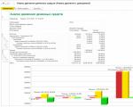
The creation of new projects involves a preliminary economic justification for their feasibility, subsequent...
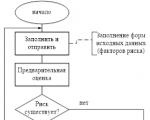
Reporting is generated by the RM, is agreed upon (approved) by the Risk Committee under the Management Board and transmitted to...

At the edge of a large, very large meadow, on a long emerald blade of grass lived a tiny Ladybug. God's little...

Nowadays, it is quite common for people to turn to the stars. With the help of a horoscope a person can find out...

Business or friendly. If you were pursuing a stranger, it means your level of trust in the female sex...

according to Freud's dream book If you dreamed about how you were fishing, it means that in real life you can hardly switch off...

Starting a family is the dream of most women. They want to have a loving husband and a bunch of kids. But it's not always...

This article contains: the most powerful prayer for divorce - information taken from all over the world, electronic...