Herring under a fur coat - a classic recipe
What would New Year be without champagne, tangerines, Olivier, aspic and everyone’s favorite “Herring under a fur coat”. With the last one...
Among physical quantities, magnetic flux occupies an important place. This article explains what it is and how to determine its size.
Formula-magnitnogo-potoka-600x380.jpg?x15027" alt="Magnetic flux formula" width="600" height="380">!}
Magnetic flux formula
This is a quantity that determines the level of the magnetic field passing through the surface. It is designated “FF” and depends on the strength of the field and the angle of passage of the field through this surface.
It is calculated according to the formula:
FF=B⋅S⋅cosα, where:
The SI unit of measurement is “weber” (Wb). 1 Weber is created by a field of 1 Tesla passing perpendicular to a surface with an area of 1 m².
Thus, the flow is maximum when its direction coincides with the vertical and is equal to “0” if it is parallel to the surface.
Interesting. The magnetic flux formula is similar to the formula by which illumination is calculated.
One of the field sources is permanent magnets. They have been known for many centuries. The compass needle was made from magnetized iron, and in Ancient Greece there was a legend about an island that attracted metal parts of ships.
Permanent magnets come in various shapes and are made from different materials:
All magnets are bipolar. This is most noticeable in rod and horseshoe devices.
If the rod is suspended from the middle or placed on a floating piece of wood or foam, it will turn in the north-south direction. The pole pointing north is called the north pole and is painted blue on laboratory instruments and designated “N.” The opposite one, pointing south, is red and labeled "S". Magnets with like poles attract, and with opposite poles they repel.
In 1851, Michael Faraday proposed the concept of closed induction lines. These lines come out of the north pole of the magnet, pass through the surrounding space, enter the south and return to the north inside the device. The lines and field strength are closest at the poles. The attractive force is also higher here.
If you put a piece of glass on the device and sprinkle iron filings on top in a thin layer, they will be located along the magnetic field lines. When several devices are placed nearby, the sawdust will show the interaction between them: attraction or repulsion.
Magnit-i-zheleznye-opilki-600x425.jpeg?x15027" alt="Magnet and iron filings" width="600" height="425">!}
Magnet and iron filings
Our planet can be imagined as a magnet, the axis of which is inclined by 12 degrees. The intersections of this axis with the surface are called magnetic poles. Like any magnet, the Earth's lines of force run from the north pole to the south. Near the poles they run perpendicular to the surface, so there the compass needle is unreliable, and other methods have to be used.
Particles of the “solar wind” have an electric charge, so when moving around them, a magnetic field appears, interacting with the Earth’s field and directing these particles along the lines of force. Thus, this field protects the earth's surface from cosmic radiation. However, near the poles, these lines are directed perpendicular to the surface, and charged particles enter the atmosphere, causing the northern lights.
In 1820, Hans Oersted, while conducting experiments, saw the effect of a conductor through which an electric current flows on a compass needle. A few days later, Andre-Marie Ampere discovered the mutual attraction of two wires through which a current flowed in the same direction.
Interesting. During electric welding, nearby cables move when the current changes.
Ampere later suggested that this was due to the magnetic induction of current flowing through the wires.
In a coil wound with an insulated wire through which electric current flows, the fields of the individual conductors reinforce each other. To increase the attractive force, the coil is wound on an open steel core. This core is magnetized and attracts iron parts or the other half of the core in relays and contactors.
Elektromagnit-1-600x424.jpg?x15027" alt="Electromagnets" width="600" height="424">!}
Electromagnets
When the magnetic flux changes, an electric current is induced in the wire. This fact does not depend on what causes this change: the movement of a permanent magnet, the movement of a wire, or a change in the current strength in a nearby conductor.
This phenomenon was discovered by Michael Faraday on August 29, 1831. His experiments showed that the EMF (electromotive force) appearing in a circuit bounded by conductors is directly proportional to the rate of change of flux passing through the area of this circuit.
Important! For an emf to occur, the wire must cross the power lines. When moving along the lines, there is no EMF.
If the coil in which the EMF occurs is connected to an electrical circuit, then a current arises in the winding, creating its own electromagnetic field in the inductor.
When a conductor moves in a magnetic field, an emf is induced in it. Its direction depends on the direction of movement of the wire. The method by which the direction of magnetic induction is determined is called the “right-hand method”.
Pravilo-pravoj-ruki-600x450.jpg?x15027" alt="Right hand rule" width="600" height="450">!}
Right hand rule
Calculating the magnitude of the magnetic field is important for the design of electrical machines and transformers.
In order to understand the meaning of the new concept of “magnetic flux”, we will analyze in detail several experiments with inducing an EMF, paying attention to the quantitative side of the observations made.
In our experiments we will use the setup shown in Fig. 2.24.
It consists of a large multi-turn coil wound, say, on a tube of thick laminated cardboard. The coil is powered from the battery through a switch and an adjusting rheostat. The amount of current installed in the coil can be judged by an ammeter (not shown in Fig. 2.24).
Inside the large coil, another small coil can be installed, the ends of which are connected to a magnetoelectric device - a galvanometer.
For clarity of the picture, part of the coil is shown cut out - this allows you to see the location of the small coil.
When the switch is closed or opened, an EMF is induced in the small coil and the galvanometer needle is thrown from the zero position for a short time.
Based on the deviation, one can judge in which case the applied EMF is greater and in which it is less.
Rice. 2.24. A device on which you can study the induction of EMF by a changing magnetic field
By noticing the number of divisions by which the arrow is thrown, one can quantitatively compare the effect produced by the induced emf.
First observation. Having inserted a small one inside the large coil, we will secure it and for now we will not change anything in their location.
Let's turn on the switch and, by changing the resistance of the rheostat connected after the battery, set a certain current value, for example
Let us now turn off the switch while observing the galvanometer. Let its discard n be equal to 5 divisions to the right:
When the 1A current is turned off.
Let's turn on the switch again and, changing the resistance, increase the current of the large coil to 4 A.
Let's let the galvanometer calm down and turn off the switch again, observing the galvanometer.
If its discard was 5 divisions when turning off the current 1 A, now when turning off 4 A, we note that the discard has increased 4 times:
When the 4A current is turned off.
Continuing such observations, it is easy to conclude that the rejection of the galvanometer, and therefore the induced EMF, increases in proportion to the increase in the switched current.
But we know that a change in current causes a change in the magnetic field (its induction), so the correct conclusion from our observation is this:
the induced emf is proportional to the rate of change of magnetic induction.
More detailed observations confirm the correctness of this conclusion.
Second observation. Let's continue observing the galvanometer's rejection, turning off the same current, say, 1-4 A. But we will change the number of turns N of the small coil, leaving its location and dimensions unchanged.
Let us assume that the galvanometer rejection
observed at (100 turns on a small coil).
How will the rejection of the galvanometer change if the number of turns is doubled?
Experience shows that
This is exactly what was to be expected.
In fact, all turns of a small coil are under the same influence of a magnetic field, and the same EMF must be induced in each turn.
Let us denote the EMF of one turn by the letter E, then the EMF of 100 turns connected in series one after the other should be 100 times greater:
At 200 turns
For any other number of turns
If the emf increases in proportion to the number of turns, then it goes without saying that the rejection of the galvanometer should also be proportional to the number of turns.
This is what experience shows. So,
the induced emf is proportional to the number of turns.
We emphasize once again that the dimensions of the small coil and its location remained unchanged during our experiment. It goes without saying that the experiment was carried out in the same large coil with the same current turned off.
Third observation. Having carried out several experiments with the same small coil while the switched current remains constant, it is easy to verify that the magnitude of the induced emf depends on how the small coil is positioned.
To observe the dependence of the induced EMF on the position of the small coil, we will improve our setup somewhat (Fig. 2.25).
To the outward end of the axis of the small coil we attach an index arrow and a circle with division (like

Rice. 2.25. A device for turning a small coil mounted on a rod passed through the walls of a large coil. The rod is connected to the index arrow. The position of the arrow on the semi-circle with divisions shows how the small coil of those that can be found on radios is located).
By turning the rod, we can now judge by the position of the index arrow the position occupied by the small coil inside the large one.
Observations show that
the greatest emf is induced when the axis of the small coil coincides with the direction of the magnetic field,
in other words, when the axes of the large and small coils are parallel.

Rice. 2.26. To the conclusion of the concept of “magnetic flux”. The magnetic field is depicted by lines drawn at the rate of two lines per 1 cm2: a - a coil with an area of 2 cm2 is located perpendicular to the direction of the field. A magnetic flux is coupled to each turn of the coil. This flux is depicted by four lines crossing the coil; b - a coil with an area of 4 cm2 is located perpendicular to the direction of the field. A magnetic flux is coupled to each turn of the coil. This flux is depicted by eight lines crossing the coil; c - a coil with an area of 4 cm2 is located obliquely. The magnetic flux associated with each of its turns is depicted by four lines. It is equal as each line depicts, as can be seen from Fig. 2.26, a and b, flow c. The flux coupled to the coil is reduced due to its tilt
This arrangement of a small coil is shown in Fig. 2.26, a and b. As the coil rotates, the emf induced in it will become less and less.
Finally, if the plane of the small coil becomes parallel to the field lines, no emf will be induced in it. The question may arise, what will happen with further rotation of the small coil?
If we rotate the coil more than 90° (relative to the initial position), then the sign of the induced emf will change. The field lines will enter the coil from the other side.
Fourth observation. It is important to make one final observation.
Let's choose a certain position in which we will place the small coil.
Let us agree, for example, to always place it in such a position that the induced EMF is as large as possible (of course, for a given number of turns and a given value of the switched-off current). Let's make several small coils of different diameters, but with the same number of turns.
We will place these coils in the same position and, turning off the current, we will observe the rejection of the galvanometer.
Experience will show us that
the induced emf is proportional to the cross-sectional area of the coils.
Magnetic flux. All observations allow us to conclude that
the induced emf is always proportional to the change in magnetic flux.
But what is magnetic flux?
First, we will talk about the magnetic flux through a flat area S forming a right angle with the direction of the magnetic field. In this case, the magnetic flux is equal to the product of the area and the induction or
here S is the area of our site, m2;; B - induction, T; F - magnetic flux, Wb.
The unit of flow is the weber.
Representing the magnetic field through lines, we can say that the magnetic flux is proportional to the number of lines piercing the area.
If the field lines are drawn so that their number on a perpendicular plane is equal to the field induction B, then the flux is equal to the number of such lines.
In Fig. 2.26 magnetic lule in is depicted by lines drawn at the rate of two lines per each line, thus corresponding to a magnetic flux of magnitude
Now, in order to determine the magnitude of the magnetic flux, it is enough to simply count the number of lines piercing the site and multiply this number by
In the case of Fig. 2.26, and the magnetic flux through an area of 2 cm2, perpendicular to the direction of the field,
In Fig. 2.26, and this area is pierced by four magnetic lines. In the case of Fig. 2.26, b magnetic flux through a transverse area of 4 cm2 at an induction of 0.2 T
and we see that the site is pierced by eight magnetic lines.
Magnetic flux coupled to a coil. When talking about induced EMF, we need to keep in mind the flux coupled to the coil.
A flow coupled to a coil is a flow that penetrates the surface bounded by the coil.
In Fig. 2.26 flux coupled to each turn of the coil, in the case of Fig. 2.26, a is equal to a in the case of Fig. 2.26, b the flow is equal to
If the area is not perpendicular, but inclined to the magnetic lines, then it is no longer possible to determine the flux simply by multiplying the area by the induction. The flux in this case is defined as the product of induction and the projection area of our site. We are talking about a projection onto a plane perpendicular to the lines of the field, or, as it were, about a shadow cast by the platform (Fig. 2.27).
However, for any shape of the site, the flow is still proportional to the number of lines passing through it, or equal to the number of single lines piercing the site.

Rice. 2.27. To the output of the site projection. Carrying out the experiments in more detail and combining our third and fourth observations, one could draw the following conclusion; the induced emf is proportional to the area of the shadow that our small coil would cast on a plane perpendicular to the field lines if it were illuminated by rays of light parallel to the field lines. This shadow is called a projection
So, in Fig. 2.26, the flux through an area of 4 cm2 at an induction of 0.2 T is equal to only (lines priced at ). Representing the magnetic field with lines is very helpful in determining the flux.
If flux Ф is linked to each of the N turns of the coil, the product NФ can be called the complete flux linkage of the coil. The concept of flux linkage can be used especially conveniently when different flows are linked to different turns. In this case, the total flux linkage is the sum of the fluxes linked to each of the turns.
A few notes about the word "flow". Why are we talking about flow? Is this word associated with the idea of some kind of flow of something magnetic? In fact, when we say “electric current,” we imagine the movement (flow) of electric charges. Is the situation the same in the case of magnetic flux?
No, when we say “magnetic flux,” we only mean a specific measure of the magnetic field (field strength times area), similar to the measure used by engineers and scientists who study the movement of fluids. When water moves, they call it the flow of the product of the speed of water and the area of the transversely located platform (the flow of water in a pipe is equal to its speed by the cross-sectional area of the pipe).
Of course, the magnetic field itself, which is one of the types of matter, is also associated with a special form of motion. We do not yet have sufficiently clear ideas and knowledge about the nature of this movement, although modern scientists know a lot about the properties of the magnetic field: the magnetic field is associated with the existence of a special form of energy, its main measure is induction, another very important measure is magnetic flux.
magnetic induction
- is the magnetic flux density at a given point in the field. The unit of magnetic induction is tesla(1 T = 1 Wb/m2).Returning to the previously obtained expression (1), we can quantitatively determine magnetic flux through a certain surface as the product of the amount of charge flowing through a conductor combined with the boundary of this surface when the magnetic field completely disappears, and the resistance of the electrical circuit through which these charges flow
.In the experiments described above with a test coil (ring), it moved away to such a distance that all manifestations of the magnetic field disappeared. But you can simply move this coil within the field and at the same time electric charges will also move in it. Let's move on to the increments in expression (1)
|
Ф + Δ Ф = r(q - Δ q) => Δ Ф = - rΔq => Δ q= -Δ Ф/ r |
where Δ Ф and Δ q- increments in flow and number of charges. The different signs of the increments are explained by the fact that the positive charge in experiments with the removal of the turn corresponded to the disappearance of the field, i.e. negative increment of magnetic flux.
Using a test turn, you can explore the entire space around a magnet or coil with current and build lines, the direction of the tangents to which at each point will correspond to the direction of the magnetic induction vector B(Fig. 3)

These lines are called magnetic induction vector lines or magnetic lines .
The space of the magnetic field can be mentally divided by tubular surfaces formed by magnetic lines, and the surfaces can be selected in such a way that the magnetic flux inside each such surface (tube) is numerically equal to one and the axial lines of these tubes can be depicted graphically. Such tubes are called single, and the lines of their axes are called single magnetic lines . A picture of a magnetic field depicted using single lines gives not only a qualitative, but also a quantitative idea of it, because in this case, the magnitude of the magnetic induction vector turns out to be equal to the number of lines passing through a unit surface area normal to the vector B, A the number of lines passing through any surface is equal to the value of the magnetic flux .
Magnetic lines are continuous and this principle can be represented mathematically as
those. magnetic flux passing through any closed surface is zero .

Expression (4) is valid for the surface s any shape. If we consider the magnetic flux passing through the surface formed by the turns of a cylindrical coil (Fig. 4), then it can be divided into surfaces formed by individual turns, i.e. s=s 1 +s 2 +...+s 8 . Moreover, in the general case, different magnetic fluxes will pass through the surfaces of different turns. So in Fig. 4, eight single magnetic lines pass through the surfaces of the central turns of the coil, and only four through the surfaces of the outer turns.
In order to determine the total magnetic flux passing through the surface of all turns, it is necessary to add up the fluxes passing through the surfaces of individual turns, or, in other words, interlocking with individual turns. For example, magnetic fluxes interlocking with the four upper turns of the coil in Fig. 4 will be equal: Ф 1 =4; Ф 2 =4; Ф 3 =6; Ф 4 =8. Also, mirror-symmetrical with the lower ones.
Flux linkage - virtual (imaginary total) magnetic flux Ψ, meshing with all turns of the coil, is numerically equal to the sum of the fluxes meshing with individual turns: Ψ = w e F m, where Ф m is the magnetic flux created by the current passing through the coil, and w e is the equivalent or effective number of coil turns. The physical meaning of flux linkage is the coupling of the magnetic fields of the coil turns, which can be expressed by the coefficient (multiplicity) of flux linkage k= Ψ/Ф = w e.
That is, for the case shown in the figure, two mirror-symmetrical halves of the coil:
|
Ψ = 2(Ф 1 + Ф 2 + Ф 3 + Ф 4) = 48 |
The virtuality, that is, the imaginary nature of the flux linkage is manifested in the fact that it does not represent a real magnetic flux, which no inductance can multiply, but the behavior of the coil impedance is such that it seems that the magnetic flux increases by a multiple of the effective number of turns, although in reality it is simple interaction of turns in the same field. If the coil increased the magnetic flux by its flux linkage, then it would be possible to create magnetic field multipliers on the coil even without current, because flux linkage does not imply the closed circuit of the coil, but only the joint geometry of the proximity of the turns.
Often the real distribution of flux linkage across the turns of a coil is unknown, but it can be assumed to be uniform and the same for all turns if the real coil is replaced by an equivalent one with a different number of turns w e, while maintaining the flux linkage value Ψ = w e F m, where Ф m- flux interlocking with the internal turns of the coil, and w e is the equivalent or effective number of coil turns. For the one considered in Fig. 4 cases w e = Ψ/Ф 4 =48/8=6.
The flow of the magnetic induction vector B through any surface. The magnetic flux through a small area dS, within which the vector B is unchanged, is equal to dФ = ВndS, where Bn is the projection of the vector onto the normal to the area dS. Magnetic flux F through the final... ... Big Encyclopedic Dictionary
MAGNETIC FLUX- (magnetic induction flux), flux F of the magnetic vector. induction B through k.l. surface. M. p. dФ through a small area dS, within the limits of which the vector B can be considered unchanged, is expressed by the product of the area size and the projection Bn of the vector onto ... ... Physical encyclopedia
magnetic flux- A scalar quantity equal to the flux of magnetic induction. [GOST R 52002 2003] magnetic flux The flux of magnetic induction through a surface perpendicular to the magnetic field, defined as the product of the magnetic induction at a given point by the area... ... Technical Translator's Guide
MAGNETIC FLUX- (symbol F), a measure of the strength and extent of the MAGNETIC FIELD. The flux through area A at right angles to the same magnetic field is Ф = mHA, where m is the magnetic PERMEABILITY of the medium, and H is the intensity of the magnetic field. Magnetic flux density is the flux... ... Scientific and technical encyclopedic dictionary
MAGNETIC FLUX- flux Ф of the magnetic induction vector (see (5)) B through the surface S normal to the vector B in a uniform magnetic field. SI unit of magnetic flux (cm) ... Big Polytechnic Encyclopedia
MAGNETIC FLUX- a value characterizing the magnetic effect on a given surface. The magnetic field is measured by the number of magnetic lines of force passing through a given surface. Technical railway dictionary. M.: State transport... ... Technical railway dictionary
Magnetic flux- a scalar quantity equal to the flux of magnetic induction... Source: ELECTRICAL ENGINEERING. TERMS AND DEFINITIONS OF BASIC CONCEPTS. GOST R 52002 2003 (approved by Resolution of the State Standard of the Russian Federation dated 01/09/2003 N 3 art.) ... Official terminology
magnetic flux- flux of magnetic induction vector B through any surface. The magnetic flux through a small area dS, within which the vector B is unchanged, is equal to dФ = BndS, where Bn is the projection of the vector onto the normal to the area dS. Magnetic flux F through the final... ... encyclopedic Dictionary
magnetic flux- , the flux of magnetic induction is the flux of the magnetic induction vector through any surface. For a closed surface, the total magnetic flux is zero, which reflects the solenoidal nature of the magnetic field, i.e. the absence in nature... Encyclopedic Dictionary of Metallurgy
Magnetic flux- 12. Magnetic flux Magnetic induction flux Source: GOST 19880 74: Electrical engineering. Basic concepts. Terms and definitions original document 12 magnetic on ... Dictionary-reference book of terms of normative and technical documentation
Let there be a magnetic field in some small region of space that can be considered uniform, that is, in this region the magnetic induction vector is constant, both in magnitude and direction.
Let us select a small area with an area ΔS, the orientation of which is specified by the unit normal vector n(Fig. 445).
rice. 445
Magnetic flux through this area ΔФ m is defined as the product of the area of the site and the normal component of the magnetic field induction vector
Where ![]()
dot product of vectors B And n;
Bn− component of the magnetic induction vector normal to the site.
In an arbitrary magnetic field, the magnetic flux through an arbitrary surface is determined as follows (Fig. 446): 
rice. 446
− the surface is divided into small areas ΔS i(which can be considered flat);
− the induction vector is determined B i on this site (which within the site can be considered permanent);
− the sum of flows through all areas into which the surface is divided is calculated
This amount is called flux of the magnetic field induction vector through a given surface (or magnetic flux).
Note that when calculating the flux, the summation is carried out over the field observation points, and not over the sources, as when using the superposition principle. Therefore, magnetic flux is an integral characteristic of the field, describing its averaged properties over the entire surface under consideration.
It is difficult to find the physical meaning of magnetic flux, as for other fields it is a useful auxiliary physical quantity. But unlike other fluxes, magnetic flux is so common in applications that in the SI system it was awarded a “personal” unit of measurement - Weber 2: 1 Weber− magnetic flux of a uniform magnetic field of induction 1 T across the area 1 m2 oriented perpendicular to the magnetic induction vector.
Now we will prove a simple but extremely important theorem about magnetic flux through a closed surface.
Previously, we established that the forces of any magnetic field are closed; it already follows from this that the magnetic flux through any closed surface is equal to zero.
Nevertheless, we present a more formal proof of this theorem.
First of all, we note that the principle of superposition is valid for magnetic flux: if a magnetic field is created by several sources, then for any surface the field flux created by a system of current elements is equal to the sum of the field fluxes created by each current element separately. This statement follows directly from the superposition principle for the induction vector and the directly proportional relationship between the magnetic flux and the magnetic induction vector. Therefore, it is sufficient to prove the theorem for the field created by a current element, the induction of which is determined by the Biot-Savarre-Laplace law. Here the structure of the field, which has axial circular symmetry, is important for us; the value of the modulus of the induction vector is unimportant.
Let us choose as a closed surface the surface of a block cut out as shown in Fig. 447. 
rice. 447
The magnetic flux is nonzero only through its two lateral faces, but these fluxes have opposite signs. Recall that for a closed surface, an outer normal is chosen, so on one of the indicated faces (the front) the flux is positive, and on the back it is negative. Moreover, the modules of these flows are equal, since the distribution of the field induction vector on these faces is the same. This result does not depend on the position of the considered block. An arbitrary body can be divided into infinitesimal parts, each of which is similar to the considered bar.
Finally, let us formulate another important property of the flow of any vector field. Let an arbitrary closed surface bound a certain body (Fig. 448). 
rice. 448
Let us divide this body into two parts, limited by parts of the original surface Ω 1 And Ω 2, and close them with a common interface between the body. The sum of the fluxes through these two closed surfaces is equal to the flux through the original surface! Indeed, the sum of the flows across the boundary (once for one body, another time for another) is equal to zero, since in each case it is necessary to take different, opposite normals (each time external). Similarly, one can prove the statement for an arbitrary partition of a body: if a body is divided into an arbitrary number of parts, then the flux through the surface of the body is equal to the sum of the fluxes through the surfaces of all parts of the partition of the body. This statement is obvious for fluid flow.
In fact, we have proven that if the flux of a vector field is zero through some surface bounding a small volume, then this flux is zero through any closed surface.
So, for any magnetic field the magnetic flux theorem is valid: the magnetic flux through any closed surface is zero Ф m = 0.
Previously, we looked at flow theorems for the fluid velocity field and the electrostatic field. In these cases, the flow through a closed surface was completely determined by point sources of the field (sources and sinks of liquid, point charges). In the general case, the presence of a non-zero flux through a closed surface indicates the presence of point field sources. Hence, The physical content of the magnetic flux theorem is the statement about the absence of magnetic charges.
If you have a good understanding of this issue and are able to explain and defend your point of view, then you can formulate the magnetic flux theorem like this: “No one has yet found the Dirac monopole.”
It should be especially emphasized that when we talk about the absence of field sources, we mean precisely point sources, similar to electric charges. If we draw an analogy with the field of a moving fluid, electric charges are like points from which fluid flows out (or flows in), increasing or decreasing its amount. The emergence of a magnetic field, due to the movement of electric charges, is similar to the movement of a body in a liquid, which leads to the appearance of vortices that do not change the total amount of liquid.
Vector fields for which the flux through any closed surface is zero received a beautiful, exotic name - solenoidal. A solenoid is a coil of wire through which electric current can be passed. Such a coil can create strong magnetic fields, so the term solenoidal means “similar to the field of a solenoid,” although such fields could be called more simply “magnetic-like.” Finally, such fields are also called vortex, similar to the velocity field of a fluid that forms all kinds of turbulent vortices in its movement.
The magnetic flux theorem is of great importance; it is often used to prove various properties of magnetic interactions, and we will encounter it several times. For example, the magnetic flux theorem proves that the induction vector of the magnetic field created by an element cannot have a radial component, otherwise the flux through a cylindrical surface coaxial with the current element would be non-zero.
We now illustrate the application of the magnetic flux theorem to calculate the magnetic field induction. Let the magnetic field be created by a ring with current, which is characterized by a magnetic moment p m. Let us consider the field near the axis of the ring at a distance z from the center, significantly larger than the radius of the ring (Fig. 449). 
rice. 449
Previously, we obtained a formula for the magnetic field induction on the axis for large distances from the center of the ring 
We will not make a big mistake if we assume that the vertical (let the axis of the ring is vertical) component of the field within a small ring of radius has the same value r, the plane of which is perpendicular to the axis of the ring. Since the vertical field component changes with distance, radial field components must inevitably be present, otherwise the magnetic flux theorem will not hold! It turns out that this theorem and formula (3) are enough to find this radial component. Select a thin cylinder with a thickness Δz and radius r, the lower base of which is at a distance z from the center of the ring, coaxial with the ring and apply the magnetic flux theorem to the surface of this cylinder. The magnetic flux through the lower base is equal to (note that the induction and normal vectors are opposite here) ![]()
Where Bz(z) z;
the flow through the upper base is
Where B z (z + Δz)− value of the vertical component of the induction vector at height z + Δz;
flow through the side surface (from axial symmetry it follows that the modulus of the radial component of the induction vector B r is constant on this surface): ![]()
According to the proven theorem, the sum of these flows is equal to zero, so the equation is valid
from which we determine the required value
It remains to use formula (3) for the vertical component of the field and carry out the necessary calculations 3 
Indeed, a decrease in the vertical component of the field leads to the appearance of horizontal components: a decrease in outflow through the bases leads to “leakage” through the side surface.
Thus, we have proven the “criminal theorem”: if less flows out of one end of a pipe than is poured into it from the other end, then somewhere they are stealing through the side surface.
1 It is enough to take the text with the definition of the flow of the electric field strength vector and change the notation (which is what is done here).
2 Named in honor of the German physicist (member of the St. Petersburg Academy of Sciences) Wilhelm Eduard Weber (1804 - 1891)
3 The most literate can see the derivative of function (3) in the last fraction and simply calculate it, but we will have to once again use the approximate formula (1 + x) β ≈ 1 + βx.

What would New Year be without champagne, tangerines, Olivier, aspic and everyone’s favorite “Herring under a fur coat”. With the last one...

Let's prepare the necessary ingredients for the cookies. The first thing to do is put the water to boil. We need...

Is it possible to register an employee for the position of financial director - chief accountant? The chief accountant claims that yes, but...

The head of a small business can easily manage the budget independently. CHECKED! If you're budgeting...
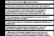
The creation of new projects involves a preliminary economic justification for their feasibility, subsequent...
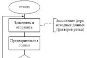
Reporting is generated by the RM, is agreed upon (approved) by the Risk Committee under the Management Board and transmitted to...

At the edge of a large, very large meadow, on a long emerald blade of grass lived a tiny Ladybug. God's little...

Nowadays, it is quite common for people to turn to the stars. With the help of a horoscope a person can find out...

Business or friendly. If you were pursuing a stranger, it means your level of trust in the female sex...

according to Freud's dream book If you dreamed about how you were fishing, it means that in real life you can hardly switch off...

The New Year's whirlwind will spin us around so quickly and rapidly that it's time to thoroughly think through the New Year's...

The article offers you some of the most delicious recipes for making vinaigrette. Vinaigrette is a delicious salad...

July 4th, 2015 , 08:33 pm Lately our Nastena has been completely giving up sweets (and thank God), but...

Fragrant, very tasty chocolate cake, it’s impossible to stop eating! The Negro’s Kiss cake is very easy to prepare,...

Let's prepare the necessary ingredients for the cookies. The first thing to do is put the water to boil. Us...

Is it possible to register an employee for the position of financial director - chief accountant? The chief accountant claims...