Herring under a fur coat - a classic recipe
What would New Year be without champagne, tangerines, Olivier, aspic and everyone’s favorite “Herring under a fur coat”. With the last one...
“Once upon a time there lived a man
twisted legs..."
From a children's book of poems.
This poem is not just about crooked legs. Everything there is twisted and crooked. And not only there. In the morning, going to work, school, or in the evening, approaching home, we do not feel the curvature of the Earth in any way (also, as it turns out, crooked). We are more hindered by all sorts of crooked bumps in our path. Therefore, the curvature of the Earth is to some extent a relative thing.
When performing geodetic work in relatively small areas, the Earth's surface can be taken as flat, and the measured distances on a flat image can be taken equal to the corresponding distances on a spherical surface. Most often, it is precisely this kind of work that has to be carried out in small areas: within a construction site, within a mine field, etc. When measuring significant distances, it is necessary to take into account the influence of the curvature of the Earth's surface. But, as will be shown later, measuring some distances requires taking into account the curvature of the Earth even for relatively small distances on its surface.
For simplicity of presentation, let us assume that the Earth is a sphere with a radius R(the radius of the Earth, represented as a sphere, is taken equal to 6371.11 km). Suppose that along the surface of the ball from the point A exactly IN the material point moves (rolls) (Fig. 2.1), while the distance S = AB which this point will travel along the surface of the ball is equal to
Where α - central angle of the arc AB(in radians).
Let's assume that the point is moving tangent to the point A to the surface of the ball and a path will pass along it S o = AB", corresponding to the motion on the surface of the ball on the way S. For value S o can be written:
. (2.2)
Difference in distances traveled ΔS = (S o - S) = R (tgα – α) and will be an error in the measured distance due to the curvature of the Earth.
For small angles α when expanding a function into a series tan α we get
, (2.3)
and after substitution into the expression for S-
, (2.4)
because the α = S/R.
Let us similarly consider the influence of the curvature of the Earth on the determination of vertical distances.
It has been mathematically established that the error (deviation) h, equal to the difference of the segments OV" And OB = R, is found through the previously accepted parameters using the formula
or, due to the small difference S And S o at small α And h, - according to the formula
. (2.6)

An estimate of possible errors when measuring vertical and horizontal distances is given in Table. 2.1.
Table 2.1
Errors in measured distances due to the curvature of the Earth
The accuracy of measuring lines in geodetic networks of higher classes is determined by a relative error of the order of 1:400000, which is practically comparable for S= 10 km (and of course more than 10 km). Up to 10 km, when measuring horizontal distances, in many cases the influence of the curvature of the Earth can be neglected.
The author apologizes for introducing the concept into the story relative error, yes and absolute error, without any necessary explanation of this concept. It turns out a concept without a concept. But this will be discussed in more detail later, but now the author, I think, correctly considered that the reader understands the word error even without defining the word. Well, the relative error is the same error, but simply expressed in a different form. For example, if the absolute error of 8 mm is divided by the measured distance of 10 km (see Table 2.1), then the following relative error will be obtained: 1/1250000.
A completely different picture is observed when assessing errors in vertical segments. This is exactly what the warning above was about. The accuracy of determining heights during geodetic work, for example, during topographic surveys, is determined by the value of 5 cm, i.e. already for distances S= 1000 m it is necessary to take into account the curvature of the Earth. If the measurement accuracy is higher, for example 5 mm or less, then taking into account the curvature of the Earth should begin for approximately distances of 250 - 300 m, which can be easily verified by reverse calculation using formula (2.6).
Rice. 4 Basic lines and planes of the observer
For orientation at sea, a system of conventional lines and planes of the observer has been adopted. In Fig. 4 shows a globe on the surface of which at a point M the observer is located. His eye is at the point A. Letter e indicates the height of the observer's eye above sea level. The line ZMn drawn through the observer's place and the center of the globe is called a plumb or vertical line. All planes drawn through this line are called vertical, and perpendicular to it - horizontal. The horizontal plane НН/ passing through the observer's eye is called true horizon plane. The vertical plane VV / passing through the observer's place M and the earth's axis is called the plane of the true meridian. At the intersection of this plane with the surface of the Earth, a large circle PnQPsQ / is formed, called observer's true meridian. The straight line obtained from the intersection of the plane of the true horizon with the plane of the true meridian is called true meridian line or the midday N-S line. This line determines the direction to the northern and southern points of the horizon. The vertical plane FF / perpendicular to the plane of the true meridian is called plane of the first vertical. At the intersection with the plane of the true horizon, it forms the E-W line, perpendicular to the N-S line and defining the directions to the eastern and western points of the horizon. Lines N-S and E-W divide the plane of the true horizon into quarters: NE, SE, SW and NW.

Fig.5. Horizon visibility range
In the open sea, the observer sees a water surface around the ship, limited by a small circle CC1 (Fig. 5). This circle is called the visible horizon. The distance De from the position of the vessel M to the visible horizon line CC 1 is called range of the visible horizon. The theoretical range of the visible horizon Dt (segment AB) is always less than its actual range De. This is explained by the fact that, due to the different density of atmospheric layers in height, a ray of light does not propagate in it rectilinearly, but along an AC curve. As a result, the observer can additionally see some part of the water surface located behind the line of the theoretical visible horizon and limited by the small circle CC 1. This circle is the line of the observer's visible horizon. The phenomenon of refraction of light rays in the atmosphere is called terrestrial refraction. Refraction depends on atmospheric pressure, temperature and humidity. In the same place on Earth, refraction can change even over the course of one day. Therefore, when calculating, the average refraction value is taken. Formula for determining the range of the visible horizon:
As a result of refraction, the observer sees the horizon line in the direction AC / (Fig. 5), tangent to the arc AC. This line is raised at an angle r above the direct ray AB. Corner r also called terrestrial refraction. Corner d between the plane of the true horizon NN / and the direction to the visible horizon is called inclination of the visible horizon.
VISIBILITY RANGE OF OBJECTS AND LIGHTS. The range of the visible horizon allows one to judge the visibility of objects located at water level. If an object has a certain height h above sea level, then an observer can detect it at a distance:
On nautical charts and in navigation manuals, the pre-calculated visibility range of lighthouse lights is given. Dk from an observer's eye height of 5 m. From such a height De equals 4.7 miles. At e, different from 5 m, an amendment should be made. Its value is equal to:
Then the visibility range of the lighthouse Dn is equal to:
The visibility range of objects calculated using this formula is called geometric or geographic. The calculated results correspond to a certain average state of the atmosphere during the daytime. When there is darkness, rain, snow or foggy weather, the visibility of objects is naturally reduced. On the contrary, under a certain state of the atmosphere, refraction can be very large, as a result of which the visibility range of objects turns out to be much greater than calculated.

Distance of the visible horizon. Table 22 MT-75:
The table is calculated using the formula:
De = 2.0809 ,
Entering the table 22 MT-75 with item height h above sea level, get the visibility range of this object from sea level. If we add to the obtained range the range of the visible horizon, found in the same table according to the height of the observer’s eye e above sea level, then the sum of these ranges will be the visibility range of the object, without taking into account the transparency of the atmosphere.
To obtain the range of the radar horizon Dp accepted selected from the table. 22 increase the range of the visible horizon by 15%, then Dp=2.3930 . This formula is valid for standard atmospheric conditions: pressure 760 mm, temperature +15°C, temperature gradient - 0.0065 degrees per meter, relative humidity, constant with altitude, 60%. Any deviation from the accepted standard state of the atmosphere will cause a partial change in the range of the radar horizon. In addition, this range, i.e. the distance from which reflected signals can be visible on the radar screen, largely depends on the individual characteristics of the radar and the reflective properties of the object. For these reasons, use the coefficient of 1.15 and the data in table. 22 should be used with caution.
The sum of the ranges of the radar horizon of the antenna Ld and the observed object of height A will represent the maximum distance from which the reflected signal can return.
Example 1.
Determine the detection range of a beacon with height h=42 m from sea level from the height of the observer's eye e=15.5 m.
Solution. From the table 22 choose:
for h = 42 m..... . Dh= 13.5 miles;
For e= 15.5 m. . . . . . De= 8.2 miles,
therefore, the detection range of the beacon
Dp = Dh+De = 21.7 miles.
The visibility range of an object can also be determined by the nomogram placed on the insert (Appendix 6). MT-75
Example 2.
Find the radar range of an object with height h=122 m, if the effective height of the radar antenna is Hd = 18.3 m above sea level.
Solution. From the table 22 choose the visibility range of the object and antenna from sea level, respectively, 23.0 and 8.9 miles. Summing these ranges and multiplying them by a factor of 1.15, the object is likely to be detected from a distance of 36.7 miles under standard atmospheric conditions.
The general shape of the Earth, as a material body, is determined by the action of internal and external forces on its particles. If the Earth were a stationary homogeneous body and subject only to internal gravitational forces, it would have the shape of a sphere. The action of centrifugal force caused by the rotation of the Earth around its axis determines the oblateness of the Earth at the poles. Under the influence of internal and external forces, the physical (topographic) surface of the Earth forms an irregular, complex shape. At the same time, on the physical surface of the Earth there are a variety of irregularities: mountains, ridges, valleys, basins, etc. It is impossible to describe such a figure using any analytical dependencies. At the same time, to solve geodetic problems in the final form, it is necessary to be based on a certain mathematically strict figure - only then is it possible to obtain calculation formulas. Based on this, the task of determining the shape and size of the Earth is usually divided into two parts:
1) establishing the shape and size of some typical figure representing the Earth in general;
2) study of deviations of the physical surface of the Earth from this typical figure.
It is known that 71% of the earth's surface is covered by seas and oceans, land – only 29%. The surface of the seas and oceans is characterized by the fact that at any point it is perpendicular to the plumb line, i.e. the direction of gravity (if the water is at rest). The direction of gravity can be set at any point and, accordingly, a surface perpendicular to the direction of this force can be constructed. A closed surface that at any point is perpendicular to the direction of gravity, i.e. perpendicular to the plumb line is called a level surface.
The level surface, which coincides with the average water level in the seas and oceans in their calm state and is mentally continued under the continents, is called the main (initial, zero) level surface. In geodesy, the general figure of the Earth is taken to be a figure limited by the main level surface, and such a figure is called a geoid (Fig. 1.1).
Due to the special complexity and geometric irregularity of the geoid, it is replaced by another figure - an ellipsoid, formed by rotating the ellipse around its minor axis RR 1 (Fig. 1.2). The dimensions of the ellipsoid were determined repeatedly by scientists from a number of countries. In the Russian Federation they were calculated under the guidance of Professor F.N. Krasovsky in 1940 and in 1946, by resolution of the Council of Ministers of the USSR, the following were approved: the semi-major axis A= 6,378,245 m, semi-minor axis b= 6,356,863 m, compression
The Earth's ellipsoid is oriented in the Earth's body so that its surface most closely matches the surface of the geoid. An ellipsoid with certain dimensions and a certain way oriented in the body of the Earth is called a reference ellipsoid (spheroid).
The largest deviations of the geoid from the spheroid are 100–150 m. In cases where, when solving practical problems, the figure of the Earth is taken to be a sphere, the radius of the sphere, equal in volume to the Krasovsky ellipsoid, is R= 6,371,110 m = 6371.11 km.
When solving practical problems, a spheroid or a sphere is taken as a typical figure of the Earth, and for small areas the curvature of the Earth is not taken into account at all. Such deviations are advisable, since geodetic work is simplified. But these deviations lead to distortions when displaying the physical surface of the Earth using the method that is commonly called in geodesy the method of projections.
The projection method in drawing up maps and plans is based on the fact that points on the physical surface of the Earth A, B and so on are projected with plumb lines onto a level surface (see Fig. 1.3, A,b). Points a, b and so on are called horizontal projections of the corresponding points of the physical surface. Then the position of these points on a level surface is determined using various coordinate systems, and then they can be plotted on a sheet of paper, i.e. a segment will be plotted on a sheet of paper ab, which is the horizontal projection of the segment AB. But, in order to determine the actual value of the segment from the horizontal projection AB, need to know the lengths aA And bB(see Fig. 1.3, b), i.e. distances from points A And IN to a level surface. These distances are called absolute heights of terrain points.
Thus, the task of drawing up maps and plans breaks down into two:
determining the position of horizontal projections of points;
determining the heights of terrain points.
When projecting points onto a plane, and not onto a level surface, distortions appear: instead of a segment ab there will be a segment a"b" instead of terrain point heights aA And bB will a"A And b"B(see Fig. 1.3, A,b).
So, the lengths of horizontal projections of segments and the heights of points will be different when projected onto a level surface, i.e. when taking into account the curvature of the Earth, and when projecting onto a plane, when the curvature of the Earth is not taken into account (Fig. 1.4). These differences will be observed in the projection lengths D S = t–S, at the heights of points D h = b"O – bO = b"O – R.

Rice. 1.3. Projection method
The problem with regard to taking into account the curvature of the Earth comes down to the following: taking the Earth as a ball with a radius R,it is necessary to determine for which largest value of the segment S the curvature of the Earth can be ignored, provided that at present the relative error ![]() is considered acceptable with the most accurate distance measurements (-1 cm per 10 km). The length distortion will be
is considered acceptable with the most accurate distance measurements (-1 cm per 10 km). The length distortion will be
D S = t – S = R tga - R a = R(tga –
a). But since S small compared to the radius of the Earth R, then for a small angle we can take ![]() . Then
. Then  . But even then
  . Respectively
  and km (rounded to the nearest 1 km).

Rice. 1.4. Scheme for solving the problem of the influence of the curvature of the Earth
on the amount of distortion in projections and heights
Consequently, a section of the spherical surface of the Earth with a diameter of 20 km can be taken as a plane, i.e. The curvature of the Earth within such an area, based on the error, can be ignored.
Distortion in the height of point D h = b"О – bО = R seca - R = R(seca – 1). Taking ![]() , we get
, we get 
 . At different values S we get:
| S, km: | 0,1; | 0,2; | 0,3; | 1; | 10; |
| D h, cm: | 0,1; | 0,3; | 0,7; | 7,8; | 78,4. |
In engineering and geodetic work, the permissible error is usually no more than 5 cm per 1 km, and therefore the curvature of the Earth should be taken into account at relatively small distances between points, about 0.8 km.
1.2. General concepts about maps, plans and profiles
The main difference between a plan and a map is that when depicting sections of the earth's surface on a plan, horizontal projections of the corresponding segments are drawn without taking into account the curvature of the Earth. When drawing maps, the curvature of the Earth must be taken into account.
Practical needs for accurate images of areas of the earth's surface are different. When drawing up projects for construction projects, they are significantly higher than during a general study of the area, geological surveys, etc.
It is known that, taking into account the permissible error when measuring distances D S= 1 cm per 10 km, a section of the spherical surface of the Earth with a diameter of 20 km can be taken as a plane, i.e. The curvature of the Earth for such a site can be ignored.
Accordingly, the creation of a plan can be schematically represented as follows. Directly on the ground (see Fig. 1.3, A) measure distances AB, BC..., horizontal angles b 1; b 2 ... and the angles of inclination of the lines to the horizon n 1, n 2 .... Then from the measured length of the terrain line, for example AB, go to the length of its orthogonal projection a"b" on a horizontal plane, i.e. determine the horizontal location of this line using the formula a"b" = AB cosn, and, decreasing by a certain number of times (scale), plot the segment a"b" on paper. Having calculated in a similar way the horizontal positions of other lines, a polygon is obtained on paper (reduced and similar to the polygon a"b"c"d"e"), which is the outline plan of the area ABCDE.
Plan – a reduced and similar image on a horizontal projection plane of a small area of the earth's surface without taking into account the curvature of the earth.
Plans are usually divided according to content and scale. If only local objects are depicted on the plan, then such a plan is called contour (situational). If the plan additionally shows the relief, then such a plan is called topographical.
Standard plan scales are 1:500; 1:1000; 1:2000; 1:5000.
Maps are usually developed for a wide area of the earth's surface, and the curvature of the earth must be taken into account. The image of a section of an ellipsoid or sphere cannot be transferred to paper without breaks. At the same time, the corresponding maps are intended to solve specific problems, for example, to determine distances, area areas, etc. When developing maps, the goal is not to completely eliminate distortions, which is impossible, but to reduce distortions and determine their values mathematically so that real values can be calculated from distorted images. For this purpose, map projections are used, which make it possible to depict the surface of a spheroid or sphere on a plane according to mathematical laws that provide measurements on a map.
Various requirements for maps have determined the presence of many map projections, which are divided into equiangular, equal-area and arbitrary. In equiangular (conformal) projections of a spheroid onto a plane, the angles of the depicted figures are preserved, but the scale changes when moving from point to point, which leads to distortion of figures of finite sizes. However, small areas of the map within which changes in scale are not significant can be considered and used as a plan.
In equal-area (equivalent) projections, the ratio of the areas of any figures on the spheroid and on the map is preserved, i.e. the scales of the areas are the same everywhere (with different scales in different directions).
In arbitrary projections, neither equiangularity nor equal area is observed. They are used for small-scale overview maps, as well as for special maps in cases where the maps have some specific useful property.
Map – constructed according to certain mathematical laws, a reduced and generalized image of the Earth’s surface on a plane.
Maps are usually divided according to content, purpose and scale.
In terms of content, maps can be general geographical and thematic, and in terms of purpose – universal and special. General geographic maps for universal purposes display the earth's surface showing all its main elements (settlements, hydrography, etc.). The mathematical basis, content and design of special maps are subject to their intended purpose (marine, aviation and many other relatively narrow-purpose maps).
Based on scale, maps are conventionally divided into three types:
large-scale (1:100,000 and larger);
medium-scale (1:200,000 – 1:1,000,000);
small-scale (smaller than 1:1,000,000).
Maps, like plans, are contour and topographic. In the Russian Federation, state topographic maps are published on a scale of 1:1,000,000 – 1:10,000.
In cases where maps or plans are used to design engineering structures, visibility in relation to the physical surface of the Earth in any direction becomes particularly important to obtain the optimal solution. For example, when designing linear structures (roads, canals, etc.) it is necessary: a detailed assessment of the steepness of the slopes in individual sections of the route, a clear understanding of the soil, ground and hydrological conditions of the area through which the route passes. Profiles provide this visibility, allowing you to make informed engineering decisions.
Profile– an image on the plane of a vertical section of the earth’s surface in a given direction. To make the unevenness of the earth's surface more noticeable, the vertical scale should be chosen larger than the horizontal one (usually 10–20 times). Thus, as a rule, the profile is not similar, but a distorted image of a vertical section of the earth's surface.
Scale
Horizontal projections of segments (see Fig. 1.3, b segments ab or a"b") when drawing up maps and plans, they are depicted on paper in a reduced form. The degree of such reduction is characterized by scale.
Scale map (plan) - the ratio of the length of a line on a map (plan) to the length of the horizontal layout of the corresponding terrain line:
 .
.
Scales can be numerical or graphic. The numerical scale is fixed in two ways.
1. As a simple fraction – the numerator is one, the denominator is the degree of reduction m, for example (or M = 1:2000).
2. In the form of a named ratio, for example, 1 cm 20 m. The expediency of such a ratio is determined by the fact that when studying the terrain on a map, it is convenient and customary to estimate the length of segments on the map in centimeters, and to represent the length of horizontal lines on the ground in meters or kilometers. To do this, the numerical scale is converted into different types of units of measurement: 1 cm of the map corresponds to such and such a number of meters (kilometers) of terrain.
Example 1. On the plan (1 cm 50 m) the distance between the points is 1.5 cm. Determine the horizontal distance between these same points on the ground.
Solution: 1.5 ´ 5000 = 7500 cm = 75 m (or 1.5 ´ 50 = 75 m).
Example 2. The horizontal distance between two points on the ground is 40 m. What will be the distance between these same points on the plan? M = 1:2000 (in 1 cm 20 m)?
Solution: see  .
.
To avoid calculations and speed up work, use graphical scales. There are two such scales: linear and transverse.
For building linear scale choose an initial segment convenient for a given scale (usually 2 cm long). This initial segment is called the base of the scale (Fig. 1.5). The base is laid on a straight line the required number of times, the leftmost base is divided into parts (usually into 10 parts). Then the linear scale is signed based on the numerical scale for which it is constructed (in Fig. 1.5, A For M = 1:25,000). Such a linear scale makes it possible to estimate a segment in a certain way with an accuracy of 0.1 fraction of the base; an additional part of this fraction has to be estimated by eye.
To ensure the required measurement accuracy, the angle between the map plane and each leg of the measuring compass (Fig. 1.5, b)should not be less than 60°, and the length of the segment should be measured at least twice. Divergence D S, m between the measurement results there should be ![]() , Where T– the number of thousands in the denominator of the numerical scale. So, for example, when measuring segments on a map M and using a linear scale, which is usually placed behind the southern side of the frame of the map sheet, discrepancies in double measurements should not exceed 1.5 ´ 10 = 15 m.
, Where T– the number of thousands in the denominator of the numerical scale. So, for example, when measuring segments on a map M and using a linear scale, which is usually placed behind the southern side of the frame of the map sheet, discrepancies in double measurements should not exceed 1.5 ´ 10 = 15 m.

Rice. 1.5. Linear scale
If the segment is longer than the constructed linear scale, then it is measured in parts. In this case, the discrepancy between the measurement results in the forward and reverse directions should not exceed , where P - number of meter settings when measuring a given segment.
For more accurate measurements use transverse scale, having an additional vertical construction on a linear scale (Fig. 1.6).
After the required number of scale bases have been set aside (also usually 2 cm long, then the scale is called normal), perpendiculars to the original line are restored and divided into equal segments (by m parts). If the base is divided into P parts and division points of the upper and lower bases are connected by inclined lines (transversals) as shown in Fig. 1.6, then the segment ![]() . Accordingly, the segment ef= 2CD;рq = 3cd etc. If m = n= 10, then cd = 0.01 base, i.e. such a transverse scale allows you to evaluate a segment in a certain way with an accuracy of 0.01 fraction of a base, an additional part of this fraction - by eye. Transverse scale, which has a base length of 2 cm and m = n = 10 is called the hundredth normal.
. Accordingly, the segment ef= 2CD;рq = 3cd etc. If m = n= 10, then cd = 0.01 base, i.e. such a transverse scale allows you to evaluate a segment in a certain way with an accuracy of 0.01 fraction of a base, an additional part of this fraction - by eye. Transverse scale, which has a base length of 2 cm and m = n = 10 is called the hundredth normal.

Rice. 1.6. Constructing a transverse scale
The transverse scale is engraved on metal rulers, which are called scales. Before using the scale ruler, you should evaluate the base and its shares according to the following diagram.
Let the numerical scale be 1:5000, the named ratio will be: 1 cm 50 m. If the transverse scale is normal (base 2 cm, Fig. 1.7), then the base will be 100 m; 0.1 base – 10 m; 0.01 bases – 1 m. The task of laying down a segment of a given length comes down to determining the number of bases, its tenths and hundredths and, if necessary, an eye-based determination of part of its smallest fraction. Let, for example, you want to set aside a segment d = 173.35 m, i.e. you need to take into the meter solution: 1 base +7 (0.1 base) +3 (0.01 base) and by eye place the legs of the meter between the horizontal lines 3 And 4 (see Fig. 1.7) so that the line AB cut off 0.35 of the space between these lines (segment DE). The inverse problem (determining the length of a segment taken into the meter solution) is accordingly solved in the reverse order. Having achieved alignment of the meter needles with the corresponding vertical and inclined lines so that both legs of the meter are on the same horizontal line, we read the number of bases and its shares ( d BG = 235.3 m).

Rice. 1.7. Transverse scale
When conducting terrain surveys to obtain plans, the question inevitably arises: what is the smallest size of terrain objects that should be displayed on the plan? Obviously, the larger the shooting scale, the smaller the linear size of such objects will be. In order for a certain decision to be made in relation to a specific scale of the plan, the concept of scale accuracy is introduced. In this case, we proceed from the following. It has been experimentally established that it is impossible to measure the distance using a compass and a scale ruler more accurately than 0.1 mm. Accordingly, scale accuracy is understood as the length of a segment on the ground corresponding to 0.1 mm on a plan of a given scale. So, if M 1:2000, then the accuracy will be:  , But d pl =
0.1 mm then d local = 2000 ´ 0.1 mm = 200 mm = 0.2 m. Consequently, on this scale (1:2000) the maximum graphic accuracy when drawing lines on the plan will be characterized by a value of 0.2 m, although the lines on the ground could be measured with higher accuracy.
, But d pl =
0.1 mm then d local = 2000 ´ 0.1 mm = 200 mm = 0.2 m. Consequently, on this scale (1:2000) the maximum graphic accuracy when drawing lines on the plan will be characterized by a value of 0.2 m, although the lines on the ground could be measured with higher accuracy.
It should be borne in mind that when measuring the relative position of contours on a plan, the accuracy is determined not by the graphical accuracy, but by the accuracy of the plan itself, where errors can average 0.5 mm due to the influence of errors other than graphic ones.
Practical part
I. Solve the following problems.
1. Determine the numerical scale if the horizontal location of a 50 m long terrain line on the plan is expressed by a segment of 5 cm.
2. The plan should display a building whose actual length is 15.6 m. Determine the length of the building on the plan in mm.
II. Construct a linear scale by drawing a line 8 cm long (see Fig. 1.5, A). Having chosen a scale base 2 cm long, set aside 4 bases, divide the leftmost base into 10 parts, digitize for three scales: ; ; .
III. Solve the following problems.
1. Lay out a segment 144 m long on paper in the three indicated scales.
2. Using the linear scale of the training map, measure the horizontal length of the three segments. Evaluate the measurement accuracy using the dependence. Here T– the number of thousands in the denominator of the numerical scale.
IV. Using a scale ruler, solve the following problems.
Put down the length of the terrain lines on paper, recording the results of the exercise in the table. 1.1.

What would New Year be without champagne, tangerines, Olivier, aspic and everyone’s favorite “Herring under a fur coat”. With the last one...

Let's prepare the necessary ingredients for the cookies. The first thing to do is put the water to boil. We need...

Is it possible to register an employee for the position of financial director - chief accountant? The chief accountant claims that yes, but...

The head of a small business can easily manage the budget independently. CHECKED! If you're budgeting...

The creation of new projects involves a preliminary economic justification for their feasibility, subsequent...
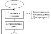
Reporting is generated by the RM, is agreed upon (approved) by the Risk Committee under the Management Board and transmitted to...

At the edge of a large, very large meadow, on a long emerald blade of grass lived a tiny Ladybug. God's little...

Nowadays, it is quite common for people to turn to the stars. With the help of a horoscope a person can find out...

Business or friendly. If you were pursuing a stranger, it means your level of trust in the female sex...

according to Freud's dream book If you dreamed about how you were fishing, it means that in real life you can hardly switch off...

The New Year's whirlwind will spin us around so quickly and rapidly that it's time to thoroughly think through the New Year's...

The article offers you some of the most delicious recipes for making vinaigrette. Vinaigrette is a delicious salad...

July 4th, 2015 , 08:33 pm Lately our Nastena has been completely giving up sweets (and thank God), but...

Fragrant, very tasty chocolate cake, it’s impossible to stop eating! The Negro’s Kiss cake is very easy to prepare,...
Let's prepare the necessary ingredients for the cookies. The first thing to do is put the water to boil. Us...

Is it possible to register an employee for the position of financial director - chief accountant? The chief accountant claims...