

Philosophical vision of the problem
The meaning of life is related to the question “What to live for”, and not to the question of how to maintain life. A person's attitude is...
MATHEMATICAL MODELS IN BIOLOGY
T.I. Volynkina
D. Skripnikova student
Federal State Educational Institution of Higher Professional Education "Oryol State Agrarian University"
Mathematical biology is the theory of mathematical models of biological processes and phenomena. Mathematical biology refers to applied mathematics and actively uses its methods. The criterion of truth in it is mathematical proof; the most important role is played by mathematical modeling using computers. Unlike purely mathematical sciences, in mathematical biology purely biological problems and problems are studied using the methods of modern mathematics, and the results have a biological interpretation. The tasks of mathematical biology are the description of the laws of nature at the level of biology and the main task is the interpretation of the results obtained during research. An example is the Hardy-Weinberg law, which proves that a population system can be predicted based on this law. Based on this law, a population is a group of self-sustaining alleles in which natural selection provides the basis. Natural selection itself is, from a mathematical point of view, an independent variable, and a population is a dependent variable, and a population is considered a number of variables that influence each other. This is the number of individuals, the number of alleles, the density of alleles, the ratio of the density of dominant alleles to the density of recessive alleles, etc. Over the past decades, there has been significant progress in the quantitative (mathematical) description of the functions of various biosystems at various levels of life organization: molecular, cellular, organ, organismal, population, biogeocenological. Life is determined by many different characteristics of these biosystems and processes occurring at the appropriate levels of system organization and integrated into a single whole during the functioning of the system.
The construction of mathematical models of biological systems became possible thanks to the exceptionally intensive analytical work of experimenters: morphologists, biochemists, physiologists, specialists in molecular biology, etc. As a result of this work, the morphofunctional schemes of various cells were crystallized, within which various physicochemical processes occur in an orderly manner in space and time and biochemical processes that form a very complex interweaving.
The second circumstance contributing to the involvement of mathematical apparatus in biology is the careful experimental determination of the rate constants of numerous intracellular reactions that determine the functions of the cell and the corresponding biosystem. Without knowledge of such constants, a formal mathematical description of intracellular processes is impossible.
The third condition that determined the success of mathematical modeling in biology was the development of powerful computing tools in the form of personal computers and supercomputers. This is due to the fact that usually the processes that control a particular function of cells or organs are numerous, covered by feedforward and feedback loops and, therefore, described by systems of nonlinear equations. Such equations cannot be solved analytically, but can be solved numerically using a computer.
Numerical experiments on models capable of reproducing a wide class of phenomena in cells, organs and the body allow us to evaluate the correctness of the assumptions made when constructing the models. Experimental facts are used as postulates of the models; the need for certain assumptions and assumptions is an important theoretical component of the modeling. These assumptions and assumptions are hypotheses that can be tested experimentally. Thus, models become sources of hypotheses, and, moreover, experimentally verifiable ones. An experiment aimed at testing a given hypothesis can refute or confirm it and thereby help refine the model. This interaction between modeling and experiment occurs continuously, leading to a deeper and more accurate understanding of the phenomenon: experiment refines the model, a new model puts forward new hypotheses, experiment refines the new model, and so on.
Currently, mathematical biology, which includes mathematical theories of various biological systems and processes, is, on the one hand, already a sufficiently established scientific discipline, and on the other hand, one of the most rapidly developing scientific disciplines, combining the efforts of specialists from various fields knowledge - mathematicians, biologists, physicists, chemists and computer science specialists. A number of disciplines of mathematical biology have been formed: mathematical genetics, immunology, epidemiology, ecology, a number of sections of mathematical physiology, in particular, mathematical physiology of the cardiovascular system.
Like any scientific discipline, mathematical biology has its own subject, methods, methods and procedures of research. As a subject of research, mathematical (computer) models of biological processes arise, which at the same time represent both an object of research and a tool for studying biological systems themselves. In connection with this dual essence of biomathematical models, they imply the use of existing and development of new methods for analyzing mathematical objects (theories and methods of the relevant branches of mathematics) in order to study the properties of the model itself as a mathematical object, as well as the use of the model for reproducing and analyzing experimental data obtained in biological experiments. At the same time, one of the most important purposes of mathematical models (and mathematical biology in general) is the ability to predict biological phenomena and scenarios for the behavior of a biosystem under certain conditions and their theoretical justification before (or even instead of) conducting corresponding biological experiments.
The main method for studying and using complex models of biological systems is a computational computer experiment, which requires the use of adequate calculation methods for the corresponding mathematical systems, calculation algorithms, technologies for developing and implementing computer programs, storing and processing the results of computer modeling. These requirements imply the development of theories, methods, algorithms and computer modeling technologies within various areas of biomathematics.
Finally, in connection with the main goal of using biomathematical models to understand the laws of functioning of biological systems, all stages of the development and use of mathematical models require mandatory reliance on the theory and practice of biological science.
MINISTRY OF EDUCATION AND SCIENCE OF THE RUSSIAN FEDERATION
FEDERAL STATE BUDGET EDUCATIONAL
INSTITUTION OF HIGHER PROFESSIONAL EDUCATION
"UDMURT STATE UNIVERSITY"
Faculty of Biology and Chemistry
TRAINING AND METODOLOGY COMPLEX
BY DISCIPLINE
MATH MODELING
BIOLOGICAL PROCESSES
Direction of training
Direction of training 020400 Biology
Name of master's program
"Biology" (Botany) 020421 m
"Biology" (Immunobiotechnology) 020422 m
"Biology" (Cell Biology) 020423 m
The place of the discipline in the structure of the master's program. Student competencies formed as a result of mastering the discipline. The purpose of mastering the discipline. The structure of the discipline by type of academic work, the relationship between topics and developed competencies. Contents of the discipline.
5.1 Topics of lecture sessions and their annotations
5.2. Practical lesson plans.
5.3. Laboratory workshop plans.
5.4. Student independent work program.
Educational technologies. Assessment tools for ongoing monitoring of progress, intermediate certification. Educational, methodological and information support of the discipline. Material and technical support of discipline.
PROCEDURE FOR APPROVAL OF THE WORK PROGRAM
Developer of the discipline's work program
Examination of the work program
Approval of the work program of the discipline
Other documents on assessing the quality of the discipline’s work program
(if available - FEPO, reviews from employers, undergraduates, etc.)
Quality Assessment Document(Name) | Document date |
1 . PLACE OF DISCIPLINE IN THE STRUCTURE OF PLO MASTER'S PROGRAM
Discipline enters the cycle the basic part of the mathematical and natural science cycle of the OOP master's program.
The discipline is addressed to 020400 Biology (qualification (degree) "Master"), first year of study.
The course is preceded by the following disciplines: computer science, natural science disciplines.
To successfully master the discipline, the following competencies must be developed:
capable of adapting and improving one’s scientific and cultural level (OK-3);
Successful completion of the course allows you to move on to studying the following disciplines: theoretical biology, synergetics, With Contemporary problems of biology, other disciplines of the mathematical and natural science cycle of the Master's program, the implementation of a master's thesis.
The course program is built according to the block-modular principle, in it sections highlighted:
2 . STUDENT COMPETENCIES FORMED
AS A RESULT OF MASTERING DISCIPLINE
· independently analyzes available information, identifies fundamental problems, poses a problem and performs field and laboratory biological research when solving specific problems in specialization using modern equipment and computing tools, demonstrates responsibility for the quality of work and the scientific reliability of the results (PC-3);
· creatively applies modern computer technologies in the collection, storage, processing, analysis and transmission of biological information (PC-6);
· independently uses modern computer technologies to solve research, production and technological problems of professional activity, to collect and analyze biological information (PC-13);
As a result of mastering the discipline, the student must:
know:
· about methods of modeling biological systems with their subsequent analysis using differential and integral calculus.
be able to:
· be able to apply the acquired knowledge in practical work;
· correctly present the results of model calculations performed.
Own:
· skills of integral and differential calculus;
· skills in working with a personal computer when using available software products for numerical modeling of biological systems.
3 . PURPOSE AND OBJECTIVES OF MASTERING THE DISCIPLINE
The purpose of mastering the discipline MATHEMATICAL MODELING OF BIOLOGICAL PROCESSES
is:
give some basic knowledge and ideas about the possibilities of practicing numerical methods of mathematical analysis, mathematical modeling, classification of mathematical models and the scope of their applicability, show what fundamental qualitative questions can be answered by a mathematical model, in the form of which knowledge about a biological object is formalized. This is achieved by including in the course basic issues of integral and differential calculus, the foundations of the mathematical apparatus of the qualitative theory of differential equations. Based on this knowledge, the main types of temporal and spatial dynamic behavior inherent in biological systems of different levels are considered. The possibilities of mathematical modeling are illustrated by examples of specific models that can be considered classic.
Objectives of mastering the discipline:
to form ideas about the applicability of numerical methods of mathematical analysis in relation to mathematical modeling of biological systems;
introduce specific mathematical models that a research biologist can apply (adapt) to his research;
expand knowledge on the use of software in modeling biological processes.
4. STRUCTURE OF DISCIPLINE BY TYPE OF STUDY WORK,
RELATIONSHIP OF TOPICS AND FORMED COMPETENCIES
Topic 1.2.
test work on the material of the previous lesson, theoretical introduction to the topic of the lesson, implementation of practical tasks.
Topic 1.3.(2 hours) Theoretical part.
List of assignments and tasks submitted for laboratory work:
Topic 1.4.(2 hours) Theoretical part.
List of assignments and tasks submitted for laboratory work: test work on the material of the previous lesson, theoretical introduction to the topic of the lesson, implementation of practical tasks.
Topic 1.5.(3 hours) Theoretical part.
List of assignments and tasks submitted for laboratory work: test work on the material of the previous lesson, theoretical introduction to the topic of the lesson, implementation of practical tasks.
Topic 1 hour) Theoretical part.
List of assignments and tasks submitted for laboratory work: test work on the material of the previous lesson, theoretical introduction to the topic of the lesson, implementation of practical tasks.
Topic 1.7.(2 hours) Theoretical part.
List of assignments and tasks submitted for laboratory work: test work on the material of the previous lesson, theoretical introduction to the topic of the lesson, implementation of practical tasks.
Topic 1.8.(2 hours) Theoretical part.
List of assignments and tasks submitted for laboratory work: test work on the material of the previous lesson, theoretical introduction to the topic of the lesson, implementation of practical tasks.
Topic 1.9.(2 hours) Theoretical part.
List of assignments and tasks submitted for laboratory work: test work on the material of the previous lesson, theoretical introduction to the topic of the lesson, implementation of practical tasks.
Topic 1.10.(2 hours) Theoretical part. Study of the stability of stationary states of second order nonlinear systems. Classical system of V. Volterra. Analytical research (determination of stationary states and their stability) and construction of phase and kinetic portraits. Using the Maxima analytical calculation package.
List of assignments and tasks submitted for laboratory work: test work on the material of the previous lesson, theoretical introduction to the topic of the lesson, implementation of practical tasks.
List of assignments and tasks submitted for laboratory work: test work on the material of the previous lesson, theoretical introduction to the topic of the lesson, implementation of practical tasks.
Topic 1.hour) Theoretical part.
List of assignments and tasks submitted for laboratory work: test work on the material of the previous lesson, theoretical introduction to the topic of the lesson, implementation of practical tasks.
5.4. Self-study program for master's students
SRS structure
Code of competence being formed | Subject | Form | Volume academic work (hours) | Educational materials |
|
PK-3, PK-6, PK-13 | Topic 1.1. The concept of a model. Objects, goals and modeling methods. Models in different sciences. Computer and mathematical models. History of the first models in biology. Modern classification of models of biological processes. Regression, simulation, qualitative models. Principles of simulation modeling and examples of models. Specifics of modeling living systems. | problem solving | SRS without teacher participation | ||
PK-3, PK-6, PK-13 | Topic 1.2. The concept of the derivative and how to find it (differentiation rules). Integral and methods for finding integrals. Solving problems on this topic. | problem solving | SRS without teacher participation | See the list of educational and methodological literature |
|
PK-3, PK-6, PK-13 | Topic 1.3. Drawing up (derivation) of a differential equation. Some techniques for solving homogeneous and inhomogeneous differential equations. Solution by the method of separable variables. Solution of a general linear differential equation by the Lagrange method. Solving problems on this topic. | problem solving | SRS without teacher participation | See the list of educational and methodological literature |
|
PK-3, PK-6, PK-13 | Topic 1.4. Drawing up (derivation) of a differential equation. The concept of solving a differential equation. Solution by the method of separable variables. Solution of a linear differential equation of general form. Stationary state. Stability of stationary states (case of one equation): definitions, analytical method for determining the type of stability. Taylor's formula. Solving problems on this topic. | problem solving | SRS without teacher participation | See the list of educational and methodological literature |
|
PK-3, PK-6, PK-13 | Topic 1.5. Analysis of some population growth models. Malthus' model. Logistic model of Verhulst. Model of a flow cultivator. Solving problems on this topic. | problem solving | SRS without teacher participation | See the list of educational and methodological literature |
|
PK-3, PK-6, PK-13 | Topic 1.6. Difference models of population growth. Analysis of the Malthus difference model (finding stationary states and analyzing them for stability). The discrete logistic Verhulst equation and its limitations for biological systems. Analysis of the discrete logistic Ricker equation (finding stationary states and analyzing them for stability). Qualitative analysis of difference models of population growth using the Lamerey diagram (ladder). Solving problems on this topic. | problem solving | SRS without teacher participation | See the list of educational and methodological literature |
|
PK-3, PK-6, PK-13 | Topic 1.7. A system of two autonomous ordinary linear differential equations (ODE). Solution of a system of two linear autonomous ODEs. Types of singular points. Solving problems on this topic. Using the Maxima analytical calculation package. | problem solving | SRS without teacher participation | ||
PK-3, PK-6, PK-13 | Topic 1.8. A system of two autonomous ordinary linear differential equations. Phase plane. Isoclins. Construction of phase portraits. Kinetic curves. Solving problems on this topic. | problem solving | SRS without teacher participation | See the list of educational and methodological literature. |
|
PK-3, PK-6, PK-13 | Topic 1.9. Analysis of some models described by a system of two autonomous ordinary linear differential equations. Analysis of the kinetic model of a system of linear differential equations describing chemical reactions. Solving problems on this topic. Using the Maxima analytical calculation package. | problem solving | SRS without teacher participation | See the list of educational and methodological literature. |
|
PK-3, PK-6, PK-13 | Topic 1.10. Study of the stability of stationary states of second-order nonlinear systems. Classical system of V. Volterra. Analytical research (determination of stationary states and their stability) and construction of phase and kinetic portraits. Using the Maxima analytical calculation package. | problem solving | SRS without teacher participation | See the list of educational and methodological literature |
|
PK-3, PK-6, PK-13 | Topic 1.11. Trigger systems. Competition. Analytical research (determination of stationary states and their stability) and construction of phase and kinetic portraits. Solving problems on this topic. | problem solving | SRS without teacher participation | See the list of educational and methodological literature. |
|
PK-3, PK-6, PK-13 | Topic 1.12. Oscillatory systems. Local model of Brusselator. Solving problems on this topic. Using the Maxima analytical calculation package. | problem solving | SRS without teacher participation | See the list of educational and methodological literature. |
Preparation for laboratory work – 12 works - 48 hours
The results of all types of SRS are assessed in points and are the basis of SRS.
When performing SRS, the educational and methodological materials specified in the corresponding section are used (see table SRS structure)
SRS control schedule
Legend: cr – test , To - colloquium, R - abstract, d – report, di – business game, rz – problem solving, chickens - course work , lr - laboratory work, dz - homework
6. EDUCATIONAL TECHNOLOGIES
When conducting classes and organizing independent work of undergraduates, traditional technologies of informative learning are used, which involve transferring information in a ready-made form, developing educational skills according to the model: the theoretical part of the laboratory work is structured as: lecture-exposition, lecture-explanation.
The use of traditional technologies ensures the formation of the cognitive (knowledge) component of the professional competencies of a research biologist.
In the process of studying the theoretical sections of the discipline and performing practical tasks, new educational teaching technologies are used: lecture-visualization.
When conducting laboratory classes the following are used:
The concept of a model. Objects, goals and modeling methods. Models in different sciences. Physical and mathematical models. History of the first models in biology. Modern classification of models of biological processes: regression, simulation, qualitative models. Examples of various models used in your area of scientific interest. Principles of simulation modeling and examples of models. Specifics of modeling living systems.
The concept of the derivative and how to find it (differentiation rules). Integral and methods for finding integrals. Solving problems on this topic.
Drawing up (derivation) of a differential equation. Some techniques for solving homogeneous and inhomogeneous differential equations. Solution by the method of separable variables. Solution of a general linear differential equation by the Lagrange method. Solving problems on this topic.
Methods for studying dynamic systems. Stationary state. Taylor's formula. Stability of stationary states (case of one equation): concept of stability, analytical method for determining the type of stability (Lyapunov method), graphical method for determining the type of stability. Solving problems on this topic.
Analysis of some population growth models. Malthus' models. Logistic model of Verhulst. Model of a flow cultivator. Solving problems on this topic.
Difference models of population growth. Analysis of the Malthus difference model (finding stationary states and analyzing them for stability). The discrete logistic Verhulst equation and its limitations for biological systems. Analysis of the discrete logistic Ricker equation (finding stationary states and analyzing them for stability). Qualitative analysis of difference models of population growth using the Lamerey diagram (ladder). Solving problems on this topic.
Analysis of models described by a system of two autonomous ordinary linear differential equations. Solution of a system of two linear autonomous ODEs. Analysis of the stability of the behavior of these models near singular points. Types of singular points. Solving problems on this topic.
A qualitative method for analyzing models described by a system of two autonomous ordinary linear differential equations. Phase plane. Isoclins. Construction of phase portraits. Kinetic curves. Solving problems on this topic.
Analysis of some models described by a system of two autonomous ordinary linear differential equations. Analysis of the kinetic model of a system of linear chemical reactions.
Study of the stability of stationary states of second-order nonlinear systems. Lyapunov's method of linearization of systems in the vicinity of a stationary state. Examples of studying the stability of stationary states of models of biological systems. Analysis of the Lotka kinetic equation (chemical reaction). Classical system of V. Volterra. Analytical research (determination of stationary states and their stability) and construction of phase and kinetic portraits.
Trigger systems. Competition. Analytical research (determination of stationary states and their stability) and construction of phase and kinetic portraits.
Oscillatory systems. Local model of Brusselator.
The main technology for assessing the level of development of competence(s) is: a point-rating system for assessing student performance (Order /01-04 "On the introduction of the Procedure for implementing a point-rating system for assessing the educational work of students at the Federal State Budgetary Educational Institution of Higher Professional Education "UdSU").
Total points = 100 points.
Attendance at classes and the student’s work during the class itself is assessed up to 15 points.
The test at the beginning of the lesson is worth up to 30 points.
Homework is graded up to 15 points.
Number of points allocated for credit up to 40 points
The discipline is considered mastered if at the stage of intermediate certification the student scored more than 14 points and the student’s final rating in the discipline for the semester is at least 61 points.
Scheme for converting points to traditional assessment
Exam (test) | The sum of points of two midterm controls, taking into account additional points |
||||||||||||||||||||
Table for converting final BRS points into the traditional grading system
Examples of test tasks, issued at the beginning of the lesson for 10-12 minutes.
Test task 1
Option 1
1) Find the derivative based on the definition of the concept of derivative: y = (1+3x)2
2) The population size is described by the equation: https://pandia.ru/text/78/041/images/image004_19.gif" width="88" height="41">
Option 3
1) Find the derivative based on the definition of the concept of derivative: y = (1+x)2
2) The population size is described by the equation: https://pandia.ru/text/78/041/images/image006_13.gif" width="90" height="45">
Option 2
Option 3
Solve the following differential equation.
Find a solution to the Cauchy problem if x(0)=1
![]()
Test task 3
Poll 3. Option 2
Solve the following differential equation.
Poll 3. Option 3
Solve the following differential equation.
Poll 3. Option 4
Solve the following differential equation.
![]()
Sample test tasksfor home use(specific texts of the assignment are issued to undergraduates through the IIAS system and on paper):
Homework 1
Recommendations.
1) Prepare a speech and attach a handwritten text with the report about an example of a physical model
2) Prepare a speech and attach a handwritten text with the report about an example of a regression model in your specialty (I can ask anyone) – 3-4 minutes – one per group. Should not be the same as another group's example.
3) Prepare a speech and attach a handwritten text with the report about an example of a simulation model in your specialty (I can ask anyone) – 3-4 minutes – one per group. Should not be the same as another group's example.
4) Using the definition of derivative, find the derivative for the expression:
y= 1+ x+ x 2
5) Find derivatives:
https://pandia.ru/text/78/041/images/image014_10.gif" width="84" height="41 src=">
https://pandia.ru/text/78/041/images/image017_9.gif" width="108" height="27 src=">.gif" width="105" height="41 src=">, Where u And A constant..gif" width="153" height="28 src=">
8) The bacterial population grows from an initial size of 1000 individuals to p(t) in the moment t(in days) according to the equation https://pandia.ru/text/78/041/images/image023_6.gif" width="106" height="41 src=">. Find p(t) for all moments t>0 if p(0)=0. How many years will it take for the proportion of those who have recovered to reach 90%?
3) Find a general solution for the following first-order equations and solve the Cauchy problem for the specified conditions:
If x(0)=2
![]() , if x(0)=1
, if x(0)=1
Homework 3
Recommendations. The assignment report is provided only in handwritten form indicating all intermediate calculations (an electronic version is not needed). All calculations must be transparent (write what you are calculating, indicate the original calculation formula, then the formula with substituted numbers, then the answer).
1) Population growth is described by the Verhulst equation. The capacity of the ecological niche for it is 1000. Plot a graph of the dynamics of the population size if it is known that the initial number is equal to: a) 10; b) 700; c) 1200. The growth rate r is 0.5. Specify the coordinates of the inflection point.
2) Expand the function f (x) into a Taylor series in the vicinity of the point 0 x up to 4th order:
f (x) = x 3 +1, x 0 = 1;
https://pandia.ru/text/78/041/images/image028_5.gif" width="114" height="46 src=">
https://pandia.ru/text/78/041/images/image030_5.gif" width="71" height="41 src=">. Find stationary states of the equation and determine their type of stability analytically (Lyapunov method) and with using a function graph f (x) :
f (x) = x 3 + 8x – 6x 2
f (x) = x 4 + 2x 3 − 15x 2
Homework 4
Recommendations. The assignment report is provided only in handwritten form indicating all intermediate calculations (an electronic version is not needed). All calculations must be transparent (write what you are calculating, indicate the original calculation formula, then the formula with substituted numbers, then the answer).
1) (1.0 points) Using the Lamerey diagram, construct a graph of population dynamics if the dependence Nt+1 = f (Nt) has the form and draw a conclusion about the sustainability of the population development.
|
|
2) (2.5 points) Construct a phase portrait for each of the systems in the vicinity of the stationary state according to the plan:
2.1) Find the coordinates of the singular (stationary) point
2.3) Using the isocline method (isocline: 0o, +45o, –45o, 90o, angles of intersection with the X and Y axes) construct a phase portrait of the system
2.4) using isoclines and based on point 2.2, draw a sketch of the phase portrait
2.5) Determine the direction of movement of the trial (figurative) point along the integral curves obtained in 2.4.
2.6) Select an arbitrary point on one of the integral curves obtained in paragraph 2.4 and construct a kinetic portrait of the system.
Master's student | Option | Master's student | Option |
3) (1.5 points) In the process of studying a certain population, the following dependence of population size on time was revealed (see data below).
1) Does the development of this population obey the Malthus equation or the Verhulst equation? Prove it.
2) If the development of a population obeys the Malthus equation, determine:
r
2.2) doubling period T.
2) If the development of the population obeys the logistic equation, determine:
2.1) the value of the Malthusian parameter r(specific reproduction rate);
2.2) resource parameter value TO
2.3) using values r And TO estimate the time after which population growth will begin to slow down.
This control and evaluation technology provides an assessment of the level of mastery of professional competencies.
8 EDUCATIONAL, METHODOLOGICAL AND INFORMATION SUPPORT
DISCIPLINES
Main literature
1. Riznichenko, on mathematical models in biology. Part 1. Description of processes in living systems over time. - M.; Izhevsk: RHD, 2002
Lectures. Methods of lecturing
Lectures are one of the main teaching methods in the discipline, which should solve the following problems:
· present the most important material of the course program, highlighting the main points;
· to develop among undergraduates the need for independent work on educational and scientific literature.
The main task of each lecture is to reveal the essence of the topic and analyze its main provisions. It is recommended to bring to the attention of undergraduates the structure of the course and its sections at the first lecture, and then indicate the beginning of each section, the essence and its objectives, and, having finished the presentation, summarize this section in order to link it with the next one.
Methodology for conducting laboratory classes
The objectives of laboratory work are:
· establishing connections between theory and practice in the form of experimental confirmation of the theory;
· training master's students in the ability to analyze the results obtained;
· control of independent work of undergraduates in mastering the course;
· training in professional skills
The goals of the laboratory workshop are best achieved if the experiment is preceded by certain preparatory extracurricular work. Therefore, the teacher is obliged to inform all undergraduates about the laboratory work schedule so that they can engage in targeted home preparation.
Before the start of the next lesson, the teacher must make sure that the master's students are ready to perform laboratory work through a short interview and checking that the master's students have prepared protocols for the work.
Successful mastery of the discipline presupposes the active, creative participation of the master's student through systematic, daily work.
Studying the discipline should begin with the development of a work program, paying special attention to the goals and objectives, structure and content of the course.
Review the notes immediately after class, marking any material in the lecture notes that is difficult to understand. Try to find answers to difficult questions using the recommended literature. If you are unable to understand the material on your own, formulate questions and seek help from your teacher at a consultation or the next lecture.
Regularly set aside time to review the material you have covered, testing your knowledge, skills and abilities using test questions.
Performing laboratory work
During class, obtain a lab schedule from your teacher. Get all the necessary methodological support.
Before visiting the laboratory, study the theory of the question proposed for research, read the manual for the relevant work and prepare a protocol for the work, in which you include:
· job title;
· preparing tables for filling with experimental observational data;
· equations of chemical reactions of transformations that will be carried out during the experiment;
· calculation formulas.
The preparation of reports should be carried out after completion of work in the laboratory or in another place designated for classes.
To prepare for defending the report, you should analyze the experimental results, compare them with known theoretical principles or reference data, summarize the research results in the form of conclusions on the work, and prepare answers to the questions given in the guidelines for performing laboratory work.
9. MATERIAL AND TECHNICAL SUPPORT OF DISCIPLINE
To conduct a computer workshop, you need a computer class that allows you to provide a separate workplace for each student. Computers must have parameters sufficient for the functioning of the programs being studied. If you use insufficiently powerful computers, you can recommend using older versions of programs or replacing some of the programs you are studying with less resource-intensive ones. Computers must have access to the Internet. Computers must have Windows XP (or older) installed, as well as a set of programs being studied (see the relevant section of paragraph 8 EDUCATIONAL, METHODOLOGICAL AND INFORMATION SUPPORT OF DISCIPLINE).
The computer class should have a large blackboard, chalk, and a cloth.
Students, graduate students, young scientists who use the knowledge base in their studies and work will be very grateful to you.
Posted on http://www.allbest.ru/
Introduction
Modern biology actively uses various branches of mathematics: probability theory and statistics, the theory of differential equations, game theory, differential geometry and set theory to formalize ideas about the structure and principles of functioning of living objects.
Many scientists have expressed the idea that a field of knowledge becomes a science only when it expresses its laws in the form of mathematical relationships. In accordance with this, the most “scientific” science is physics - the science of the fundamental laws of nature, mathematics for it is a natural language. In biology, where individual living systems are the subject of study, the situation is more complicated. Only in our century have experimental biochemistry, biophysics, molecular biology, microbiology, and virology appeared, which study phenomena reproducible in vitro and actively use physical, chemical and mathematical methods.
Due to the individuality of biological phenomena, we speak specifically about mathematical models in biology (and not just about mathematical language). The word model here emphasizes the fact that we are talking about abstraction, idealization, and a mathematical description, rather, not of the living system itself, but of some qualitative characteristics of the processes occurring in it. At the same time, it is possible to make quantitative predictions, sometimes in the form of statistical patterns. In some cases, for example, in biotechnology, mathematical models, as in engineering, are used to develop optimal production modes.
1. Classes of problems and mathematical apparatus
When developing any model, it is necessary to determine the object of modeling, the purpose of modeling and the means of modeling. In accordance with the object and goals, mathematical models in biology can be divided into three large classes. The first - regression models, includes empirically established dependencies (formulas, differential and difference equations, statistical laws) that do not pretend to reveal the mechanism of the process being studied. Let us give two examples of such models.
1. The relationship between the number of anchovy spawners S and the number of juveniles from each spawning spawner in a large simulation model of the dynamics of the Azov Sea fish stock is expressed as an empirical formula (Gorstko et al, 1984)
Here S is the number of fingerlings (pieces) for each spawning spawner; x is the number of anchovy producers that came from the Black Sea to the Azov Sea in the spring (billion pieces); - standard deviation.
1. The rate of oxygen absorption by leaf litter can be fairly well described by the formula for the logarithm of the oxygen absorption rate:
Here Y is the oxygen uptake measured in µl(0.25 g)-1h-1.; D is the number of days during which the samples were kept; B is the percentage of moisture in the samples; T is temperature measured in degrees C.
This formula provides unbiased estimates for the rate of oxygen uptake over the entire range of days, temperatures and humidity observed in the experiment, with a standard deviation in oxygen uptake of =0.3190.321.
(From the book: D. Jeffers "Introduction to systems analysis: application in ecology", M., 1981)
Coefficients in regression models are usually determined using procedures for identifying model parameters from experimental data. In this case, the sum of squared deviations of the theoretical curve from the experimental one for all measurement points is most often minimized. Those. The model coefficients are selected in such a way as to minimize the functionality:
Here i is the number of the measurement point; xe - "experimental values of variables; xt - theoretical values of variables; a1, a2... - parameters to be estimated; wi - "weight" of the i-th measurement; N - number of measurement points.
The second class is simulation models of specific complex living systems, which, as a rule, take into account as much as possible the available information about the object. Simulation models are used to describe objects at various levels of organization of living matter - from biomacromolecules to models of biogeocenoses. In the latter case, models should include blocks describing both living and “inert” components (See Mathematical ecology). A classic example of simulation models are molecular dynamics models, in which the coordinates and momenta of all atoms that make up a biomacromolecule and the laws of their interaction are specified. A computer-computed picture of the “life” of a system allows one to trace how physical laws are manifested in the functioning of the simplest biological objects - biomacromolecules and their environment. Similar models, in which the elements (building blocks) are no longer atoms, but groups of atoms, are used in modern computer technology for the design of biotechnological catalysts and drugs that act on certain active groups of membranes of microorganisms, viruses, or perform other targeted actions.
Simulation models are created to describe physiological processes. Occurring in vital organs: nerve fiber, heart, brain, gastrointestinal tract, bloodstream. They play “scenarios” of processes occurring normally and in various pathologies, and study the influence of various external influences, including medications, on the processes. Simulation models are widely used to describe the production process of plants and are used to develop an optimal regime for growing plants in order to obtain maximum yield, or obtain the most evenly distributed fruit ripening over time. Such developments are especially important for expensive and energy-intensive greenhouse farming.
2. High-quality (basic) models
In any science, there are simple models that can be analyzed analytically and have properties that make it possible to describe a whole range of natural phenomena. Such models are called basic. In physics, the classic basic model is the harmonic oscillator (a ball - a material point - on a spring without friction). Basic models, as a rule, are studied in detail in various modifications. In the case of an oscillator, the ball can be in a viscous medium, experience periodic or random influences, for example, energy pumping, etc. After the essence of the processes on such a basic model has been thoroughly mathematically studied, by analogy the phenomena occurring in much more complex ones become clear real systems. For example, the relaxation of confirmational states of a biomacromolecule is considered similarly to an oscillator in a viscous medium. Thus, due to their simplicity and clarity, basic models become extremely useful in studying a wide variety of systems.
All biological systems at various levels of organization, ranging from biomacromolecules up to populations, are thermodynamically nonequilibrium, open to flows of matter and energy. Therefore, nonlinearity is an integral property of basic systems of mathematical biology. Despite the huge diversity of living systems, we can highlight some of the most important qualitative properties inherent in them: growth, self-limitation of growth, ability to switch - existence in two or more stationary modes, self-oscillating modes (biorhythms), spatial heterogeneity, quasistochasticity. All these properties can be demonstrated using relatively simple nonlinear dynamic models, which act as basic models of mathematical biology.
3. Unlimited growth. Exponential growth. Autocatalysis
mathematical biology molecular population
All models are based on certain assumptions. The model built on the basis of these assumptions becomes an independent mathematical object that can be studied using an arsenal of mathematical methods. The value of a model is determined by how well the model's characteristics correspond to the properties of the modeled object. One of the fundamental assumptions underlying all growth models is that the rate of growth of a population, be it a population of hares or a population of cells, is proportional to the rate of growth. This assumption is based on the well-known fact that the most important characteristic of living systems is their ability to reproduce. For many unicellular organisms or cells that make up cellular tissues, this is simply division, that is, doubling the number of cells after a certain time interval, called the characteristic division time. For complexly organized plants and animals, reproduction occurs according to a more complex law, but in the simplest model it can be assumed that the rate of reproduction of a species is proportional to the number of this species.
Mathematically, this is written using a differential equation linear with respect to the variable x, which characterizes the number (concentration) of individuals in the population:
Here R in the general case can be a function of both the number itself and time, or depend on other external and internal factors.
The assumption that the rate of population growth is proportional to its size was expressed back in the 18th century by Thomas Robert Malthus (1766-1834) in the book “On Population Growth” (1798). According to law (1), if the proportionality coefficient R=r=const (as Malthus assumed), the number will grow exponentially without limit.
In his works, Malthus discusses the implications of this law in light of the fact that the production of food and other goods grows linearly, and therefore a population growing exponentially is doomed to starvation.
For most populations, there are limiting factors, and for one reason or another, population growth stops. The only exception is the human population, which throughout historical time has been growing even faster than exponentially. (See Mathematical ecology, section Human population growth). Malthus's research had a great influence on both economists and biologists. In particular, Charles Darwin writes in his diaries that the assumptions underlying Malthus's model and the proportionality of the population growth rate of its size seem very convincing, and from this follows unlimited exponential growth in numbers. At the same time, none of the populations in nature grows indefinitely. Therefore, there are reasons preventing such growth. Darwin sees one of these reasons in the struggle of species for existence.
The law of exponential growth is valid at a certain stage of growth for populations of cells in tissue, algae or bacteria in culture. In models, a mathematical expression that describes an increase in the rate of change of a quantity with an increase in this quantity itself is called the autocatalytic term (auto - self, catalysis - modification of the reaction rate, usually acceleration, with the help of substances that do not take part in the reaction) Thus, autocatalysis is "self-acceleration " reactions.
4. Limited growth. Verhulst equation
The basic model describing limited growth is Verhulst's model (1848):
Here the parameter K is called “population capacity” and is expressed in units of number (or concentration). It does not have any simple physical or biological meaning and is systemic in nature, that is, determined by a number of different circumstances, including restrictions on the amount of substrate for microorganisms, the available volume for a population of tissue cells, the food supply or shelters for higher animals.
The graph of the dependence of the right side of equation (2) on the size x and the population size on time is presented in Fig. 1 (a and b).
Rice. 1 Limited growth. Dependence of the growth rate on the number (a) and number on time (b) for the logistic equation
In recent decades, the Verhulst equation has experienced a second youth. The study of the discrete analogue of equation (2) revealed completely new and remarkable properties. Let's consider the population size at successive points in time. This corresponds to the actual procedure for counting individuals (or cells) in a population. In its simplest form, the dependence of the number at time step number n+1 on the number of the previous step n can be written as:
The time behavior of the variable xn can be not only of limited growth, as was the case for the continuous model (2), but also be oscillatory or quasistochastic (Fig. 2).
Rice. 2 Type of function of the dependence of the number at the next step on the number at the previous step (a) and the behavior of the number over time (b) for different values of the parameter r: 1 - limited growth; 2 - fluctuations, 3 - chaos
The type of behavior depends on the value of the intrinsic growth rate constant r. Curves representing the dependence of the population value at a given time (t+1) on the population value at the previous time t are presented in Fig. 2 on the left. On the right are curves of population dynamics - the dependence of the number of individuals in a population on time. From top to bottom, the value of the intrinsic growth rate parameter r increases.
The nature of population dynamics is determined by the shape of the curve of dependence F(t+1) on F(t). This curve reflects the change in the rate of population growth from the population itself. For all presented in Fig. 2 on the left of the curves, this speed increases at small numbers, and decreases, and then becomes zero at large numbers. The dynamic type of population growth curve depends on how quickly growth occurs at small numbers, i.e. is determined by the derivative (the tangent of the slope of this curve) at zero, which is determined by the coefficient r - the value of its own growth rate. For small r(r<3) численность популяции стремится к устойчивому равновесию. Когда график слева становится более крутым, устойчивое равновесие переходит в устойчивые циклы. По мере увеличения численности длина цикла растет, и значения численности повторяются через 2, 4, 8,..., 2n поколений. При величине параметра r>5.370 there is a chaotization of decisions. At sufficiently large r, the population dynamics exhibit chaotic bursts (outbreaks in the number of insects).
Equations of this type provide a good description of the population dynamics of seasonally reproducing insects with non-overlapping generations. At the same time, some fairly simply measurable characteristics of populations demonstrating quasi-stochastic behavior are of a regular nature. In a sense, the more chaotic the behavior of a population, the more predictable it is. For example, at large x, the flash amplitude can be directly proportional to the time between flashes.
Discrete description has proven to be productive for systems of a wide variety of natures. The apparatus for representing the dynamic behavior of a system on a plane in coordinates allows one to determine whether the observed system is oscillatory or quasistochastic. For example, the presentation of electrocardiogram data made it possible to establish that the contractions of the human heart are normally irregular, but during attacks of angina or in a pre-infarction state, the rhythm of heart contraction becomes strictly regular. This “tightening” of the regime is a protective reaction of the body in a stressful situation and indicates a threat to the life of the system.
Note that solving difference equations is the basis for modeling any real biological processes. The richness of the dynamic behavior of model trajectories of difference equations is the basis for their successful application to describe complex natural phenomena. At the same time, the limited nature of the parametric regions of existence of a certain type of regime serves as an additional basis for assessing the adequacy of the proposed model.
Even more interesting mathematical objects are obtained if we rewrite equation (3) in the form:
and consider the constant c in the complex domain. This produces objects called Mandelbrot sets. You can read more about these sets in the book “The Beauty of Fractals” (Images of Complex Dynamic Systems), where their numerous colorful images are also given. Do these objects have a biological interpretation that has a deeper meaning, or are they just a beautiful “surprise” that the underlying system gives us? There is no definitive answer to this question yet.
5. Substrate restrictions. Monod and Michaelis-Menten models
One of the reasons for growth limitation may be lack of food (substrate limitation in the language of microbiology). Microbiologists have long noticed that under conditions of substrate limitation, the growth rate increases in proportion to the concentration of the substrate, and if there is enough substrate, it reaches a constant value determined by the genetic capabilities of the population. For some time, the population grows exponentially until the growth rate begins to be limited by any other factors. This means that the dependence of the growth rate R in formula (1) on the substrate can be described as:
Here KS is a constant equal to the substrate concentration at which the growth rate is half the maximum. 0 is the maximum growth rate, equal to the value of r in formula (2). This equation was first written by a major French biochemist. Jacques Monod (1912-1976). Together with Francois Jacob, he developed ideas about the role of transport ribonucleic acid (mRNA) in the cell reproduction apparatus. In developing the idea of gene complexes, which they called operons, Jacob and Monod postulated the existence of a class of genes that regulate the functioning of other genes by influencing the synthesis of transfer RNA. This mechanism of gene regulation was subsequently fully confirmed for bacteria, for which both scientists (as well as Andre Lvov) were awarded the Nobel Prize in 1965. Below we consider the famous model of gene regulation of the synthesis of two enzymes, called the trigger model of Jacob and Monod.
Jacques Monod was also a philosopher of science and an extraordinary writer. In his famous book “Chance and Necessity,” 1971, Monod expresses thoughts about the randomness of the emergence of life and evolution, as well as the role of man and his responsibility for the processes occurring on Earth.
It is curious that the Monod model (5) coincides in form with the Michaelis-Menten equation (1913), which describes the dependence of the rate of an enzymatic reaction on the concentration of the substrate, provided that the total number of enzyme molecules is constant and significantly less than the number of substrate molecules:
Here KM is the Michaelis constant, one of the most important quantities for enzymatic reactions, determined experimentally, having the meaning and dimension of the substrate concentration at which the reaction rate is equal to half the maximum.
The Michaelis-Menten law is derived from the equations of chemical kinetics and describes the rate of product formation in accordance with the scheme:
The similarity of equations (5) and (6) is not accidental. The Michaelis-Menten formula (5) reflects deeper patterns of the kinetics of enzymatic reactions, which in turn determine the vital activity and growth of microorganisms, described by the empirical formula (5).
6. Basic interaction model. Competition. Selection.
Biological systems interact with each other at all levels, be it the interaction of biomacromolecules in the process of biochemical reactions, or the interaction of species in populations. Interaction can occur in structures, then the system can be characterized by a certain set of states, this happens at the level of subcellular, cellular and organismal structures. The kinetics of processes in structures in mathematical models is usually described using systems of equations for the probabilities of states of complexes.
In the case when the interaction occurs randomly, its intensity is determined by the concentration of the interacting components and their mobility by generalized diffusion. These are the ideas adopted in basic models of species interaction. A classic book that discusses mathematical models of the interaction of species is Vito Volterra’s book “The Mathematical Theory of the Struggle for Existence” (1931). The book is structured as a mathematical treatise, it postulates in mathematical form the properties of biological objects and their interactions, and then these interactions are studied as mathematical objects. It was with this work of V. Volterra that modern mathematical biology and mathematical ecology began.
Vito Volterra (1860-1940) gained worldwide fame for his work in the field of integral equations and functional analysis. In addition to pure mathematics, he was always interested in the application of mathematical methods in biology, physics, and social sciences. During his years serving in the Air Force in Italy, he worked a lot on issues of military equipment and technology (ballistics, bombing, echolocation problems). This man combined the talent of a scientist and the temperament of an active politician, a principled opponent of fascism. He was the only Italian senator to vote against the transfer of power to Mussolini. When Volterra worked in France during the years of the fascist dictatorship in Italy, Mussolini, wanting to win over the world-famous scientist, offered him various high positions in fascist Italy, but was always decisively refused. Volterra's anti-fascist position led him to renounce his chair at the University of Rome and his membership in Italian scientific societies.
V. Volterra became seriously interested in issues of population dynamics in 1925 after conversations with the young zoologist Umberto D'Ancona, the future husband of his daughter, Louise. D'Ancona, while studying the statistics of slave markets in the Adriatic, established an interesting fact: when during the First World War Since the war (and immediately after it), the intensity of fishing has sharply decreased, the relative share of predatory fish in the catch has increased. This effect was predicted by the predator-prey model proposed by Volterra. We will look at this model below. In fact, this was the first success of mathematical biology.
Volterra suggested, by analogy with statistical physics, that the intensity of interaction is proportional to the probability of encounter (the probability of collision of molecules), that is, the product of concentrations. This and some other assumptions (See Population dynamics) made it possible to construct a mathematical theory of interaction between populations of the same trophic level (competition) or different trophic levels (predator-prey).
The systems studied by Volterra consist of several biological species and a food supply that is used by some of the species in question. The following assumptions are formulated about the system components.
1. Food is either available in unlimited quantities, or its supply is strictly regulated over time.
2. Individuals of each species die off in such a way that a constant proportion of existing individuals die per unit time.
3. Predatory species eat prey, and per unit time the number of prey eaten is always proportional to the probability of meeting individuals of these two species, i.e. the product of the number of predators and the number of prey.
4. If there is food in unlimited quantities and several species that are capable of consuming it, then the share of food consumed by each species per unit time is proportional to the number of individuals of this species, taken with a certain coefficient depending on the species (models of interspecific competition).
5. If a species feeds on food available in unlimited quantities, the increase in the number of the species per unit of time is proportional to the number of the species.
6. If a species feeds on food available in limited quantities, then its reproduction is regulated by the rate of food consumption, i.e. per unit time, the increase is proportional to the amount of food eaten.
The listed hypotheses make it possible to describe complex living systems using systems of ordinary differential equations, on the right sides of which there are sums of linear and bilinear terms. As is known, such equations also describe systems of chemical reactions.
Indeed, according to Volterra's hypotheses, the rate of extinction of each species is proportional to the number of species. In chemical kinetics, this corresponds to a monomolecular reaction of the decomposition of a certain substance, and in a mathematical model, it corresponds to negative linear terms on the right sides of the equations. According to the concepts of chemical kinetics, the rate of the bimolecular reaction of interaction between two substances is proportional to the probability of collision of these substances, i.e. the product of their concentration. In the same way, according to Volterra’s hypotheses, the rate of reproduction of predators (death of prey) is proportional to the probability of encounters between predator and prey individuals, i.e. the product of their numbers. In both cases, bilinear terms appear in the model system on the right-hand sides of the corresponding equations. Finally, the linear positive terms on the right-hand sides of the Volterra equations, corresponding to the growth of populations under unlimited conditions, correspond to the autocatalytic terms of chemical reactions. This similarity of equations in chemical and environmental models allows us to apply the same research methods for mathematical modeling of population kinetics as for systems of chemical reactions. It can be shown that Voltaire’s equations can be obtained not only from the local “meeting principle”, which originates from statistical physics, but also from the mass balance of each of the components of the cenosis and the energy flows between these components.
Let us consider the simplest of Volterra models, the model of selection based on competitive relations. This model works when considering competitive interactions of any nature, biochemical compounds of various types of optical activity, competing cells, individuals, populations. Its modifications are used to describe competition in the economy.
Let there be two completely identical species with the same reproduction rate, which are antagonists, that is, when they meet, they oppress each other. The model of their interaction can be written as:
According to this model, the symmetrical state of coexistence of both species is unstable; one of the interacting species will necessarily die out, while the other will multiply indefinitely.
The introduction of a restriction on the substrate (type 5) or a systemic factor limiting the number of each species (type 2) makes it possible to construct models in which one of the species survives and reaches a certain stable number. They describe the Gause principle of competition, known in experimental ecology, according to which only one species survives in each ecological niche.
In the case where species have different intrinsic growth rates, the coefficients for the autocatalytic terms on the right-hand sides of the equations will be different, and the phase portrait of the system becomes asymmetrical. With different ratios of parameters in such a system, it is possible both the survival of one of the two species and the extinction of the second (if mutual oppression is more intense than the self-regulation of numbers), and the coexistence of both species, in the case where mutual oppression is less than the self-limitation of the numbers of each species.
Rice. 4 Scheme of the synthesis of two enzymes Jacob and Monod (a) and phase portrait of the trigger systems (b)
Another classic trigger system is the Jacob and Monod model of alternative synthesis of two enzymes. The synthesis scheme is shown in Fig. 4a. The gene regulator of each system synthesizes an inactive repressor. This repressor, combining with the product of the opposite enzyme synthesis system, forms an active complex. The active complex, reversibly reacting with a region of the structural gene operon, blocks mRNA synthesis. Thus, the product of the second system, P2, is a corepressor of the first system, and P1 is a corepressor of the second. In this case, one, two or more product molecules can participate in the process of corepression. Obviously, with this nature of interactions, when the first system operates intensively, the second will be blocked, and vice versa. A model of such a system was proposed and studied in detail at the school of prof. D.S. Chernavsky After appropriate simplifications, the equations describing the synthesis of products P1 and P2 have the form:
Here P1, P2 are the concentrations of products, the values A1, A2, B1, B2 are expressed through the parameters of their systems. The exponent m shows how many molecules of the active repressor (combinations of product molecules with molecules of the inactive repressor, which is expected to be in excess) bind to the operon to block mRNK synthesis.
The phase portrait of the system (image of the trajectories of the system under different initial conditions on the coordinate plane, along the axes of which the values of the system variables are plotted), for m=2 is shown in Fig. 4b. It has the same appearance as the phase portrait of a system of two competing types. The similarity indicates that the basis of the system's ability to switch is competition - species, enzymes, states.
Rice. 5 Model of chemical reactions Trays. Phase portrait of the system for parameter values corresponding to damped oscillations
7. Classic models Trays and Volterra
The first understanding that intrinsic rhythms are possible in an energy-rich system due to the specific interaction of its components came after the appearance of the simplest nonlinear models of interaction - chemical substances in the Lotka equations, and the interaction of species - in Volterra models.
The Lotka equation was discussed by him in 1926 in a book and describes the system of the following chemical reactions
In a certain volume, substance A is present in excess. Molecules of A are converted at a certain constant rate into molecules of substance X (zero-order reaction). Substance X can be converted into substance Y, and the rate of this reaction is greater, the higher the concentration of substance Y - a second-order reaction. In the diagram this is reflected by the backward arrow above the y symbol. The Y molecules, in turn, decompose irreversibly, resulting in the formation of substance B (a first-order reaction).
Let's write a system of equations describing the reaction:
Here X, Y, B are the concentrations of chemical components. The first two equations of this system do not depend on B, so they can be considered separately. At certain parameter values, damped oscillations are possible in the system.
The basic model of undamped oscillations is the classical Volterra equation, which describes the interaction of predator-prey species. As in competition models (8), species interactions are described according to the principles of chemical kinetics: the rate of loss of prey (x) and the rate of gain of predators (y) are assumed to be proportional to their product
In Fig. Figure 6 shows a phase portrait of the system, along the axes of which the numbers of prey and predators are plotted - (a) and the kinetics of the numbers of both species - the dependence of numbers on time - (b). It can be seen that the numbers of predators and prey fluctuate in antiphase.
Rice. 6 Volterra predator-prey model, describing undamped fluctuations in numbers. A. Phase portrait. B. Dependence of the number of prey and predator on time
The Volterra model has one significant drawback. The oscillation parameters of its variables change with fluctuations in the parameters and variables of the system. Such a system is called non-rough.
This drawback is eliminated in more realistic models. Modification of the Volterra model taking into account the limitation of the substrate in the Monod form (equation 5) and taking into account the self-limitation of numbers (as in equation 2) leads to a model studied in detail by A.D. Bazykin in the book “Biophysics of Interacting Populations” (1985).
System (11 is a kind of centaur, composed of basic equations (1, 2, 5, 10) and combining their properties. Indeed, with small numbers and in the absence of a predator, the prey (x) will multiply according to the exponential law (1). Predator ( y) in the absence of prey, they will also die out exponentially. If there are many individuals of a particular species, in accordance with the basic model (2), the system Verhulst factor is triggered (the term -Ex2 in the first equation, and -My2 - in the second). Intensity of species interaction is considered proportional to the product of their numbers (as in model (10)) and is described in the Monod form (model 5). Here, the role of the substrate is played by the prey species, and the role of microorganisms is played by the predator species. Thus, model (11) took into account the properties basic models (1), (2), (5), (10).
But model (11) is not just the sum of the properties of these models. With its help, it is possible to describe much more complex types of behavior of interacting species: the presence of two stable stationary states, damped fluctuations in numbers, etc. At certain parameter values, the system becomes self-oscillating. In it, over time, a regime is established in which the variables change periodically with a constant period and amplitude, regardless of the initial conditions.
8. Waves of life
So far we have talked about basic models of the behavior of living systems over time. The desire for growth and reproduction leads to distribution in space, occupation of a new area, and expansion of living organisms. Life spreads just like flame across the steppe during a steppe fire. This metaphor reflects the fact that fire (in the one-dimensional case, the spread of flame along a fuse) is described using the same basic model as the spread of a species. The PKP (Petrovsky-Kolmogorov-Piskunov) model, famous in combustion theory, was first proposed by them in 1937 precisely in a biological formulation as a model of the distribution of the dominant species in space. All three authors of this work are leading Russian mathematicians. Academician Ivan Georgievich Petrovsky (1901-1973) - author of fundamental works on the theory of differential equations, algebra, geometry, mathematical physics, was the rector of Moscow State University for more than 20 years. M.V. Lomonosov. (1951-1973). Andrei Nikolaevich Kolmogorov (1903--) head of the Russian mathematical school in probability theory and function theory, author of fundamental works on mathematical logic, topology, theory of differential equations, information theory, organizer of school and university mathematical education, wrote several works based on biological productions. In particular, in 1936, he proposed and studied in detail a generalized model of predator-prey species interaction (corrected and expanded version 1972). (See Population dynamics)
Let us consider the formulation of the problem of the distribution of a species in an active environment rich in energy (food). Let at any point on the line r>0 the reproduction of the species be described by the function f(x) = x(1-x). At the initial moment of time, the entire area to the left of zero is occupied by species x, the concentration of which is close to unity. To the right of zero is empty territory. At time t=0, the species begins to spread (diffuse) to the right with a diffusion constant D. The process is described by the equation:
At t>0 in such a system, a wave of concentrations begins to propagate into the region r>0, which is the result of two processes: random movement of individuals (diffusion of particles) and reproduction, described by the function f(x). Over time, the wave front moves to the right, and its shape approaches a certain limiting shape. The speed of wave movement is determined by the diffusion coefficient and the shape of the function f(x), and for the function f(x), equal to zero at x=0 and x=1 and positive at intermediate points, it is expressed by a simple formula: =2Df"(0).
The study of spatial movement in the predator-prey model (10) shows that in such a system, in the case of unlimited space, waves of “flight and pursuit” will propagate, and in a limited space, stationary spatially inhomogeneous structures (dissipative structures), or autowaves, will be established, depending on system parameters.
9. Autowaves and dissipative structures. Basic Brusselator model
The one-dimensional model (14) discussed above shows that the interaction of a nonlinear chemical reaction and diffusion leads to non-trivial regimes. Even more complex behavior can be expected in two-dimensional models that describe the interaction of system components. The first such model was studied by Turing in a paper entitled "The Chemical Basis of Morphogenesis." Alan M. Turing (1912-1954) English mathematician and logician, became famous for his work on computer logic and automata theory. In 1952, he published the first part of a study devoted to the mathematical theory of the formation of structures in an initially homogeneous system, where chemical reactions simultaneously occur, including autocatalytic processes accompanied by energy consumption, and passive transfer processes - diffusion. This research was left unfinished because he committed suicide while under the influence of depressants, which he was forced to treat in prison, where he was serving time on charges of homosexuality.
Turing's work became a classic; its ideas formed the basis of the modern theory of nonlinear systems, the theory of self-organization and synergetics. The system of equations is considered:
Equations of this type are called reaction-diffusion equations. In linear systems, diffusion is a process that leads to equalization of concentrations throughout the reaction volume. However, in the case of nonlinear interaction of variables x and y, instability of a homogeneous stationary state may arise in the system and complex spatiotemporal regimes such as autowaves or dissipative structures may form - stationary in time and spatially inhomogeneous distributions of concentrations, the existence of which is maintained in active media due to consumption energy of the system in dissipation processes. The condition for the appearance of structures in such systems is the difference in the diffusion coefficients of the reagents, namely, the presence of a short-range “activator” with a low diffusion coefficient and a long-range “inhibitor” with a large diffusion coefficient.
Such regimes in a two-component system were studied in detail using a basic model called the “Brussellator” (Prigogine and Lefebvre, 1968), named after the Brussels school of thought led by I. R. Prigogine, in which these studies were most intensively carried out.
Ilya Romanovich Prigozhin (born 1917 in Moscow) - worked in Belgium all his life. Since 1962, he has been director of the International Solvay Institute of Physical Chemistry in Brussels, and since 1967, director of the Center for Statistical Mechanics and Thermodynamics at the University of Texas (USA).
In 1977, he received the Nobel Prize for his work on nonlinear thermodynamics, in particular on the theory of dissipative structures - structures that are stable in time and inhomogeneous in space. Prigogine is the author and co-author of a number of books ["Thermodynamic theory of structure, stability and fluctuations", "Order from chaos", "Arrow of time", etc.], in which he develops the mathematical, physico-chemical, biological and philosophical ideas of the theory self-organization in nonlinear systems, explores the causes and patterns of the birth of “order from chaos” in energy-rich systems open to flows of matter and energy, far from thermodynamic equilibrium, under the influence of random fluctuations.
The classic Brusselator model looks like
and describes a hypothetical scheme of chemical reactions:
The key stage is the transformation of two molecules x and one molecule y into x, the so-called trimolecular reaction. Such a reaction is possible in processes involving enzymes with two catalytic centers. The nonlinearity of this reaction, combined with the processes of diffusion of matter, provides the possibility of spatiotemporal regimes, including the formation of spatial structures in an initially homogeneous system of morphogenesis.
Conclusion
Modern mathematical biology uses various mathematical apparatus to model processes in living systems and formalize the mechanisms underlying biological processes. Simulation models allow computers to simulate and predict processes in nonlinear complex systems, which are all living systems that are far from thermodynamic equilibrium. Basic models of mathematical biology in the form of simple mathematical equations reflect the most important qualitative properties of living systems: the possibility of growth and its limitations, the ability to switch, oscillatory and stochastic properties, spatiotemporal inhomogeneities. These models are used to study the fundamental possibilities of the spatiotemporal dynamics of the behavior of systems, their interactions, changes in the behavior of systems under various external influences - random, periodic, etc. Any individual living system requires deep and detailed study, experimental observation and the construction of its own model, the complexity of which depends on the object and the purposes of the modeling.
Literature
1. Volterra V. Mathematical theory of the struggle for existence. M., Nauka, 1976, 286 p.
2. Peitgen H.-O., Richter P.H. The beauty of fractals. Images of complex dynamic systems. M., Mir, 1993, 176 p.
3. Riznichenko G.Yu., Rubin A.B. Mathematical models of biological production processes. M., Ed. Moscow State University, 1993, 301 p.
4. Romanovsky Yu.M., Stepanova N.V., Chernavsky D.S. Mathematical biophysics. M., Nauka, 1984, 304 p.
5. Rubin A.B., Pytyeva N.F., Riznichenko G.Yu. Kinetics of biological processes. M., MSU., 1988
6. Svirezhev Yu.M., Logofet. Stability of biological communities M., Nauka, 1978, 352c
7. Bazykin A.D. Biophysics of interacting populations. M., Nauka, 1985, 165 p.
8. J.D. Murray "Mathematical Biology", Springer, 1989, 1993.
Posted on Allbest.ru
...Specifics of using mathematical models in biology. An example of determining the relationship between the quantity and quality of offspring. Features of simulation and basic models for describing limited growth, competition, selection and waves of life of organisms.
abstract, added 10/09/2013
Determination of the specific growth rate of a bacterial population. Solution of a first order differential equation. Finding general and particular solutions, constant C. Substituting known numbers into the equation. Calculation of bacterial population size after 4 hours.
presentation, added 03/23/2014
Subject of study: molecular biology. Requirements for solving problems of establishing the sequence of nucleotides in DNA, mRNA, tRNA anticodons, the specifics of calculating the number of hydrogen bonds, the length of DNA and RNA. Protein biosynthesis. Energy exchange.
presentation, added 05/05/2014
General characteristics of the science of biology. Stages of development of biology. Discovery of the fundamental laws of heredity. Cell theory, laws of heredity, achievements of biochemistry, biophysics and molecular biology. Question about the functions of living matter.
test, added 02/25/2012
Morphological characteristics of grouse. Species habitat, lifestyle, nutrition, reproduction, growth and development. Features of the seasonal change of feather cover. Dynamics of grouse numbers. Similarities and differences in the biology of the studied grouse species.
course work, added 02/12/2015
Dynamic characteristics of the population: fertility, mortality, survival. Spatial distribution of individuals making up populations. Consideration of population fluctuations as an auto-regulated process. Number of places available to live.
presentation, added 03/25/2015
Identification of the general nature of the distribution and location of concentration of wild boars in the North-West Caucasus. Determination of size and density, age structure and sexual population. Consideration of the behavioral characteristics of wild boars on feeding grounds.
thesis, added 07/18/2014
Methodology of modern biology. Philosophical and methodological problems of biology. Stages of transformation of ideas about the place and role of biology in the system of scientific knowledge. The concept of biological reality. The role of philosophical reflection in the development of the life sciences.
abstract, added 01/30/2010
Electrophoresis is one of the most important methods for separating and analyzing the components of substances in chemistry, biochemistry and molecular biology. Electrophoresis of proteins in polyacrylamide and agarose gel. Equipment for capillary electrophoresis.
abstract, added 08/31/2014
A study of the biography and scientific work of Charles Darwin, the founder of evolutionary biology. Substantiation of the hypothesis of human origin from an ape-like ancestor. Basic provisions of evolutionary teaching. The scope of natural selection.
Gomel, 2003
Developed by: Starodubtseva M.N., Kuznetsov B.K.
Textbook on the topic “Mathematical modeling of biological processes”
The manual contains two laboratory works introducing medical students to the basics of mathematical modeling of biological processes, one of them (two lessons) is implemented in the Mathcad computer algebra system. The first work, “Modeling the functioning of the cardiovascular system,” examines mathematical modeling of biological processes, including models of the functioning of the cardiovascular system. A systematic approach to modeling the functioning of complex objects, the principles of constructing systems of differential equations that describe the behavior of a biological object, as well as concepts such as stable and unstable states, bifurcations, oscillators, and synchronization of processes are considered. The practical part of the work contains an algorithm for calculating blood circulation parameters at rest and after exercise using experimental data and methods for their statistical analysis. The second work, related to computer modeling, contains a description of the user interface, the input language of the Mathcad system, basic calculation methods (calculating arithmetic expressions, finding derivatives of functions, integrals, solving differential equations and systems of differential equations), the basics of plotting, some statistical functions ( calculating the average value, standard deviation, finding the linear regression equation and correlation coefficient).
For 1st year students of medical higher educational institutions of all faculties.
Reviewers:
Cherenkevich S. N.,
Professor, Doctor of Biology, Head of the Department of Biophysics, Faculty of Physics, Belarusian State University,
Asenchik O. D.,
Candidate of Physical and Mathematical Sciences, Head of the Department of Information Technologies, Gomel State Technical University. P. O. Sukhoi.
Approved by the Scientific and Methodological Council of the Institute as a teaching aid _____________ 2003, protocol No. ____ on the topic: “Mathematical modeling of biological processes”
Ó Gomel State Medical Institute, 2003
Subject: Mathematical modeling of biological
processes
Mathematical modeling of biological processes.
Simulation of cardiovascular functioning
systems
Target: To study modern models of the cardiovascular system and show by their example the effectiveness of using the modeling method to assess the condition and identify characteristic features of the behavior of complex biological objects.
1.1. Theory issues
1.1.1. Mathematical modeling of biological processes. Biophysics of complex systems.
The functioning of a complex biological system, including the cardiovascular system, is the result of the interaction of its constituent elements and the processes occurring in it. It should be borne in mind that according to the general principle of an ascending hierarchy of types of movement (mechanical - physical - chemical - biological - social), the biological form of movement cannot be completely reduced to the mechanical, physical or chemical form of movement, and biological systems cannot be fully described from the standpoint of any one of these forms of movement. These forms of movement can serve as models of the biological form of movement, that is, its simplified images.
It is possible to find out the basic principles of regulating the processes of a complex biological system by first constructing a mechanical, physical or chemical model of the system, and then constructing their mathematical models, that is, finding the mathematical functions that describe these models, including equations (creating mathematical models). The lower the level of the hierarchy, the simpler the model, the more factors of the real system are excluded from consideration.
Modeling is a method in which the study of some complex object (process, phenomenon) is replaced by the study of its simplified analogue - a model. In biophysics, biology and medicine, physical, chemical, biological and mathematical models are widely used. For example, the flow of blood through vessels is modeled by the movement of fluid through pipes (physical model). A biological model is simple biological objects, convenient for experimental research, on which the properties of real, more complex biological systems are studied. For example, the patterns of occurrence and propagation of action potentials along nerve fibers were studied using a biological model—the giant squid axon.
A mathematical model is a set of mathematical objects and relationships between them, reflecting the properties and characteristics of a real object that are of interest to the researcher. An adequate mathematical model can only be constructed using specific data and ideas about the mechanisms of complex processes. After construction, the mathematical model “lives” according to its internal laws, the knowledge of which allows us to identify the characteristic features of the system under study (see diagram in Fig. 1.1.). The simulation results form the basis for managing processes of any nature.
Biological systems, in fact, are extremely complex structural and functional units.

Rice. 1.1. Scheme of a systematic approach to modeling a biological object.
Most often, mathematical models of biological processes are specified in the form of differential or difference equations, but other types of model representations are also possible. After the model is built, the task is reduced to studying its properties using methods of mathematical deduction or through machine modeling.
When studying a complex phenomenon, several alternative models are usually proposed. The qualitative correspondence of these models to the object is checked. For example, they establish the presence of stable stationary states in the model and the existence of oscillatory modes. The model that best matches the system under study is chosen as the main one. The selected model is specified in relation to the specific system under study. Numerical values of the parameters are set based on experimental data.
The process of searching for a mathematical model of a complex phenomenon can be divided into stages, the sequence and interconnection of which is reflected in the diagram in Fig. 1.2.

Rice. 1. 2. Scheme of searching for a mathematical model.
Stage 1 corresponds to the collection of data available at the beginning of the study about the object being studied.
At stage 2, a basic model (system of equations) is selected from possible alternative models based on qualitative characteristics.
At stage 3, the model parameters are identified from experimental data.
At stage 4, the behavior of the model is verified using independent experimental data. To do this, it is often necessary to carry out additional experiments.
If the experimental data taken to verify the model “does not fit” into the model, it is necessary to analyze the situation and put forward other models, study the properties of these new models, and then conduct experiments that allow one to conclude that one of them is preferable (step 5).
We have already said that the mathematical approach to the study of certain phenomena of the real world usually begins with the creation of corresponding general concepts, that is, with the construction of mathematical models that have the properties that are essential for us of the systems and processes that we study. We also mentioned the difficulties associated with the construction of such models in biology, difficulties caused by the extreme complexity of biological systems. However, despite these difficulties, the “model” approach to biological problems is now successfully developing and has already brought certain results. We will look at some models related to various biological processes and systems.
Speaking about the role of models in biological research, it is important to note the following. Although we understand the term “model” in an abstract sense - as a certain system of logical concepts, and not as a real physical device, a model is still something significantly more than a simple description of a phenomenon or a purely qualitative hypothesis, in which there is still enough room for different kind of ambiguities and subjective opinions. Let us recall the following example, dating back to the rather distant past. At one time, Helmholtz, while studying hearing, put forward the so-called resonance theory, which looked plausible from a purely qualitative point of view. However, quantitative calculations carried out later, taking into account the real values of the masses, elasticity and viscosity of the components that make up the auditory system, showed the inconsistency of this hypothesis. In other words, the attempt to transform a purely qualitative hypothesis into an exact model that allows its investigation by mathematical methods immediately revealed the inconsistency of the original principles. Of course, if we have built a certain model and even obtained good agreement between this model and the results of the corresponding biological experiment, this does not yet prove the correctness of our model. Now, if, based on the study of our model, we can make some predictions about the biological system that we are modeling, and then confirm these predictions with a real experiment, then this will be much more valuable evidence in favor of the correctness of the model.
But let's move on to specific examples.
One of the first, if not the very first, work on mathematical modeling of biological processes should be considered the work of Leonhard Euler, in which he developed the mathematical theory of blood circulation, considering, to a first approximation, the entire circulatory system as consisting of a reservoir with elastic walls, peripheral resistance and a pump. These ideas of Euler (as well as some of his other works) were at first completely forgotten, and then revived in later works of other authors.
A fairly old and well-known, but nevertheless very remarkable model in biology is the Mendelian theory of heredity. This model, based on probability theoretical concepts, is that the chromosomes of the parent cells contain certain sets of characteristics, which during fertilization are combined independently and randomly. Subsequently, this basic idea underwent very significant clarifications; for example, it was discovered that different signs are not always independent of each other; if they are associated with the same chromosome, then they can only be transmitted in a certain combination. Further, it was discovered that different chromosomes do not combine independently, but there is a property called chromosome affinity, which violates this independence, etc. Currently, theoretical-probabilistic and statistical methods have very widely penetrated into genetic research and even the term “mathematical genetics” "received full citizenship rights. Currently, intensive work is being carried out in this area; many results have been obtained that are interesting both from a biological and from a purely mathematical point of view. However, the very basis of these studies is the model that was created by Mendel more than 100 years ago.
One of the most interesting objects of physiological research is muscle. This object is very accessible, and the experimenter can carry out many studies simply on himself, having only relatively simple equipment. The functions that a muscle performs in a living organism are also quite clear and definite. Despite all this, numerous attempts to construct a satisfactory model of muscle function have not yielded definitive results. It is clear that although a muscle can stretch and contract like a spring, their properties are completely different, and even to the very first approximation, a spring cannot be considered as a semblance of a muscle. For a spring, there is a strict relationship between its elongation and the load applied to it. This is not the case for a muscle: a muscle can change its length while maintaining tension, and vice versa, change the traction force without changing its length. Simply put, at the same length, a muscle can be relaxed or tense.
Among the various operating modes possible for a muscle, the most significant are the so-called isotonic contraction (i.e., a contraction in which the muscle tension remains constant) and isometric tension, in which the length of the muscle does not change (both ends are fixed). Studying a muscle in these modes is important for understanding the principles of its operation, although under natural conditions muscle activity is neither purely isotonic nor purely isometric.
Various mathematical formulas have been proposed to describe the relationship between the speed of isotonic muscle contraction and the magnitude of the load. The most famous of them is the so-called characteristic Hill equation. It looks like
(P+a)V=b(P 0 -P),
- speed of contraction, a, b And P 0- permanent.Other well-known formulas for describing the same relationship are Ober's equation
P = P 0 e- V⁄P ±F
and the Polissar equation
V=const (A 1-P/P 0 - B 1-P/P 0).
Hill's equation has become widespread in physiology; it gives a fairly good agreement with experiment for the muscles of a wide variety of animals, although in fact it represents the result of a "fit" rather than an inference from some model. Two other equations, which give approximately the same dependence over a fairly wide range of loads as the Hill equation, were obtained by their authors from certain ideas about the physicochemical mechanism of muscle contraction. There are a number of attempts to construct a model of muscle work, considering the latter as some combination of elastic and viscous elements. However, there is still no sufficiently satisfactory model that reflects all the main features of muscle work in various modes.
Nerve cells, or neurons, are the “working units” that make up the nervous system and to which the animal or human body owes all its abilities to perceive external signals and control various parts of the body. A characteristic feature of nerve cells is that such a cell can be in two states - rest and excitation. In this, nerve cells are similar to elements such as radio tubes or semiconductor triggers, from which the logical circuits of computers are assembled. Over the past 15-20 years, many attempts have been made to model the activity of the nervous system, based on the same principles on which the work of general-purpose computers is based. Back in the 40s, American researchers McCulloch and Pitts introduced the concept of a “formal neuron,” defining it as an element (the physical nature of which does not matter) equipped with a certain number of “excitatory” and a certain number of “inhibitory” inputs. This element itself can be in two states - “rest” or “excitement”. An excited state occurs if the neuron receives a sufficient number of excitatory signals and there are no inhibitory signals. McCulloch and Pitts showed that with the help of circuits composed of such elements, it is possible, in principle, to implement any of the types of information processing that occur in a living organism. This, however, does not mean at all that we have thereby learned the actual principles of the nervous system. First of all, although nerve cells are characterized by the “all or nothing” principle, i.e. the presence of two clearly defined states - rest and excitation, it does not at all follow that our nervous system, like a universal computer, uses a binary digital code consisting of zeros and ones. For example, in the nervous system, frequency modulation apparently plays a significant role, that is, the transmission of information using the length of time intervals between impulses. In general, in the nervous system, apparently, there is no such division of information encoding methods into “digital” discrete) and “analog” (continuous), which is available in modern computer technology.
In order for a system of neurons to work as a whole, it is necessary that there be certain connections between these neurons: impulses generated by one neuron must arrive at the inputs of other neurons. These connections can have a correct, regular structure, or they can be determined only by statistical patterns and be subject to certain random changes. In currently existing computing devices, no randomness in connections between elements is allowed, however, there are a number of theoretical studies on the possibility of constructing computing devices based on the principles of random connections between elements. There are quite serious arguments in favor of the fact that the connections between real neurons in the nervous system are also largely statistical, and not strictly regular. However, opinions on this matter differ.
In general, the following can be said about the problem of modeling the nervous system. We already know quite a lot about the peculiarities of the work of neurons, that is, those elements that make up the nervous system. Moreover, with the help of systems of formal neurons (understood in the sense of McCulloch and Pitts or in some other sense), simulating the basic properties of real nerve cells, it is possible to simulate, as already mentioned, very diverse ways of processing information. Nevertheless, we are still quite far from a clear understanding of the basic principles of the functioning of the nervous system and its individual parts, and, consequently, from creating its satisfactory model *.
* (If we can create some kind of system that can solve the same problems as some other system, this does not mean that both systems work according to the same principles. For example, you can numerically solve a differential equation on a digital computer by giving it the appropriate program, or you can solve the same equation on an analog computer. We will get the same or almost the same results, but the principles of information processing in these two types of machines are completely different.)
Vision is one of the main channels through which we receive information about the outside world. The well-known expression - it is better to see once than to hear a hundred times - is also true, by the way, from a purely informational point of view: the amount of information that we perceive through vision is incomparably greater than that perceived by other senses. This importance of the visual system for a living organism, along with other considerations (specificity of functions, the possibility of conducting various studies without any damage to the system, etc.) stimulated its study and, in particular, attempts at a model approach to this problem.
The eye is an organ that serves as both an optical system and an information processing device. From both points of view, this system has a number of amazing properties. The eye's ability to adapt to a very wide range of light intensities and to correctly perceive all colors is remarkable. For example, a piece of chalk in a poorly lit room reflects less light than a piece of coal placed in bright sunlight, yet in each of these cases we perceive the colors of the corresponding objects correctly. The eye conveys relative differences in illumination intensities well and even “exaggerates” them somewhat. Thus, a gray line on a bright white background seems darker to us than a solid field of the same gray color. This ability of the eye to emphasize contrasts in illumination is due to the fact that visual neurons have an inhibitory effect on each other: if the first of two neighboring neurons receives a stronger signal than the second, then it has an intense inhibitory effect on the second, and the difference in the output of these neurons is the intensity is greater than the difference in the intensity of the input signals. Models consisting of formal neurons connected by both excitatory and inhibitory connections have attracted the attention of both physiologists and mathematicians. There are both interesting results and unsolved questions here.
Of great interest is the mechanism by which the eye perceives different colors. As you know, all shades of colors perceived by our eyes can be represented as combinations of three primary colors. Typically, these primary colors are red, blue and yellow, corresponding to wavelengths of 700, 540 and 450 Å, but this choice is not unambiguous.
The “three-color” nature of our vision is due to the fact that the human eye has three types of receptors, with maximum sensitivity in the yellow, blue and red zones, respectively. The question of how we distinguish a large number of color shades with the help of these three receptors is not very simple. For example, it is not yet clear enough what exactly this or that color is encoded in our eye: the frequency of nerve impulses, the localization of the neuron that predominantly reacts to a given shade of color, or something else. There are some model ideas about this process of perception of shades, but they are still quite preliminary. There is no doubt, however, that here, too, systems of neurons connected to each other by both excitatory and inhibitory connections should play a significant role.
Finally, the eye is also very interesting as a kinematic system. A series of ingenious experiments (many of them were carried out in the laboratory of the physiology of vision of the Institute for Problems of Information Transmission in Moscow) established the following, at first glance, unexpected fact: if some image is motionless relative to the eye, then the eye does not perceive it. Our eye, when examining an object, literally “feels” it (these eye movements can be accurately recorded using appropriate equipment). The study of the motor apparatus of the eye and the development of corresponding model representations are quite interesting both in themselves and in connection with other (optical, informational, etc.) properties of our visual system.
To summarize, we can say that we are still far from creating completely satisfactory models of the visual system that well describe all its basic properties. However, a number of important aspects and principles of its operation are already quite clear and can be modeled in the form of computer programs for a computer or even in the form of technical devices.
One of the very characteristic properties of many living tissues, primarily nervous tissue, is their ability to excite and transfer excitation from one area to another. About once a second, a wave of excitement runs through our heart muscle, causing it to contract and drive blood throughout the body. Excitation along nerve fibers, spreading from the periphery (sensory organs) to the spinal cord and brain, informs us about the outside world, and in the opposite direction there are excitation commands that prescribe certain actions to the muscles.
Excitation in a nerve cell can occur on its own (as they say, “spontaneously”), under the influence of an excited neighboring cell, or under the influence of some external signal, say, electrical stimulation coming from some current source. Having passed into an excited state, the cell remains in it for some time, and then the excitement disappears, after which a certain period of cell immunity to new stimuli begins - the so-called refractory period. During this period, the cell does not respond to signals received by it. Then the cell returns to its original state, from which a transition to a state of excitation is possible. Thus, the excitation of nerve cells has a number of clearly defined properties, starting from which it is possible to construct an axiomatic model of this phenomenon. Further, purely mathematical methods can be used to study this model.
Ideas about such a model were developed several years ago in the works of I.M. Gelfand and M.L. Tsetlin, which were then continued by a number of other authors. Let us formulate an axiomatic description of the model in question.
By “excitable medium” we mean a certain set X elements (“cells”) having the following properties:
1.Each element can be in one of three states: rest, excitement and refractoriness;
2. From each excited element, excitation spreads through many elements at rest at a certain speed v;
3.If the item X hasn't been excited for some specific time T(x), then after this time it spontaneously goes into an excited state. Time T(x) called the period of spontaneous activity of the element X. This does not exclude the case when T(x)= ∞, i.e. when spontaneous activity is actually absent;
4. The state of excitement lasts for some time τ (which may depend on X), then the element moves for a while R(x) into a refractory state, after which a state of rest sets in.
Similar mathematical models arise in completely other areas, for example, in the theory of combustion, or in problems of the propagation of light in an inhomogeneous medium. However, the presence of a “refractory period” is a characteristic feature of biological processes.
The described model can be studied either by analytical methods or by implementing it on a computer. In the latter case, we are, of course, forced to assume that the set X(excitable medium) consists of a certain finite number of elements (in accordance with the capabilities of existing computer technology - on the order of several thousand). For analytical research it is natural to assume X some continuous variety (for example, consider that X- this is a piece of plane). The simplest case of such a model is obtained if we take X some segment (a prototype of a nerve fiber) and assume that the time during which each element is in an excited state is very short. Then the process of sequential propagation of impulses along such a “nerve fiber” can be described by a chain of ordinary first-order differential equations. Already in this simplified model, a number of features of the propagation process that are also found in real biological experiments are reproduced.
The question of the conditions for the occurrence of so-called fibrillation in such a model active medium is very interesting from both a theoretical and applied medical point of view. This phenomenon, observed experimentally, for example in the heart muscle, consists in the fact that instead of rhythmic coordinated contractions, random local excitations appear in the heart, devoid of periodicity and disrupting its functioning. The first theoretical study of this problem was undertaken in the work of N. Wiener and A. Rosenbluth in the 50s. Currently, work in this direction is being intensively carried out in our country and has already yielded a number of interesting results.

The meaning of life is related to the question “What to live for”, and not to the question of how to maintain life. A person's attitude is...

A mushroom is a living organism that forms a separate kingdom of the same name. For a long time they were classified as part of the plant kingdom. But in...

For lovers of “quiet” hunting, mushroom season begins in early summer and lasts until late autumn. And rarely do they...
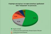
Aleshnikova, V.I. Use of professional consultants. - M.: Infra-M, 1999. - 240 p. 2. Beich, E....

Orange juice. The symbolic meaning of orange juice in dream books is pleasure and temptation. Quite often we...

We most often overcome all kinds of difficulties encountered along the path of life. Of course, for this we make...

This year your patron Neptune will be in your constellation and this is a good sign, because you will...

1993 who? 1993 is the year of which animal? — According to the Chinese horoscope, 1873, 1933, 1993 belonged to the years of the Black...

Wave-particle duality of light means that light simultaneously has the properties of continuous...

The role of biology is enormous in our world. Although it is not one of the priority subjects, most schoolchildren and...
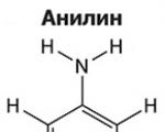
Amines are organic derivatives of ammonia containing an NH 2 amino group and an organic radical. In general...
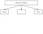
How to answer questions in Part BThe second part of the social studies work consists of 7 tasks with a short answer....

Form TORG-15 is drawn up in the case when during transportation, movement between and within the warehouse, when...

Nutritionists say that for good health and a slim figure, you must include snacks in your...

A mushroom is a living organism that forms a separate kingdom of the same name. For a long time they were classified as a kingdom...

For lovers of “quiet” hunting, mushroom season begins in early summer and lasts until late autumn. And rarely do they...